Working with Data#
This example shows how to work with the data of a loaded test system, including parameters and variables.
import andes
from andes.utils.paths import get_case

andes.config_logger()
To show all the rows and columns, change the pandas configuration with
import pandas as pd

pd.options.display.max_columns = None
pd.options.display.max_rows = None
Let's load the Kundur's system.
Load System from an ANDES XLSX File#
The ANDES xlsx file is the best supported format. Other formats can be converted to the xlsx format.
See the link below for more about format conversion. https://github.com/curent/andes/blob/master/README.md#format-converter
As previously shown, test cases can be loaded with andes.run():
ss = andes.run(get_case('kundur/kundur_full.xlsx'),
               default_config=True)  # one can remove `default_config=True` to use custom config file
Working directory: "/home/hacui/repos/andes/examples"
> Loaded generated Python code in "/home/hacui/.andes/pycode".
Parsing input file "/home/hacui/repos/andes/andes/cases/kundur/kundur_full.xlsx"...
Input file parsed in 0.1394 seconds.
System internal structure set up in 0.0319 seconds.
-> System connectivity check results:
  No islanded bus detected.
  System is interconnected.
  Each island has a slack bus correctly defined and enabled.

-> Power flow calculation
           Numba: Off
   Sparse solver: KLU
 Solution method: NR method
Power flow initialized in 0.0036 seconds.
0: |F(x)| = 14.9282832
1: |F(x)| = 3.608627841
2: |F(x)| = 0.1701107882
3: |F(x)| = 0.002038626956
4: |F(x)| = 3.745104027e-07
Converged in 5 iterations in 0.0074 seconds.
Report saved to "kundur_full_out.txt" in 0.0010 seconds.
-> Single process finished in 0.3582 seconds.
Alternatively, one can load a test case without setting up using andes.load(..., setup=False). Note that setup=False option.
It is useful to apply parameter changes to an existing test case.
ss = andes.load(get_case('kundur/kundur_full.xlsx'),
                default_config=True,
                setup=False)
Working directory: "/home/hacui/repos/andes/examples"
> Reloaded generated Python code of module "pycode".
Parsing input file "/home/hacui/repos/andes/andes/cases/kundur/kundur_full.xlsx"...
Input file parsed in 0.1263 seconds.
For example, we can toggle the connectivity status u of Line_3 to 0 using
ss.Line.alter('u', 'Line_3', 0)
When done, remember to set up the system before running calculation routines:
ss.setup()

ss.PFlow.run()
System internal structure set up in 0.0366 seconds.
-> System connectivity check results:
  No islanded bus detected.
  System is interconnected.
  Each island has a slack bus correctly defined and enabled.

-> Power flow calculation
           Numba: Off
   Sparse solver: KLU
 Solution method: NR method
Power flow initialized in 0.0049 seconds.
0: |F(x)| = 14.9282832
1: |F(x)| = 3.579044433
2: |F(x)| = 0.119268955
3: |F(x)| = 0.03278820195
4: |F(x)| = 2.880943096e-05
5: |F(x)| = 3.93747257e-11
Converged in 6 iterations in 0.0122 seconds.
Report saved to "kundur_full_out.txt" in 0.0016 seconds.
True
After setting up the system, adding or removing devices are not yet allowed.
Load System from PSS/E RAW and DYR Files#
ANDES supports loading systems from PSS/E RAW and DYR files.
The PSS/E v32 raw format is best supported.
Note that this feature is experimental. We try out best to support this format, but the compatibility is not guaranteed.
raw_path = get_case('kundur/kundur.raw')
dyr_path = get_case('kundur/kundur_full.dyr')
The raw file is passed to the positional argument, whereas the dyr file is passed to addfile.
ss = andes.run(raw_path, addfile=dyr_path, default_config=True)
Working directory: "/home/hacui/repos/andes/examples"
> Reloaded generated Python code of module "pycode".
Parsing input file "/home/hacui/repos/andes/andes/cases/kundur/kundur.raw"...
  MODIFIED KUNDUR'S TWO-AREA TEST SYSTEM, DISTRIBUTED WITH ANDES
  SEE THE BOOK "POWER SYSTEM STABILITY AND CONTROL" FOR ORIGINAL DATA
Input file parsed in 0.0047 seconds.
Parsing additional file "/home/hacui/repos/andes/andes/cases/kundur/kundur_full.dyr"...
Addfile parsed in 0.0912 seconds.
System internal structure set up in 0.0310 seconds.
-> System connectivity check results:
  No islanded bus detected.
  System is interconnected.
  Each island has a slack bus correctly defined and enabled.

-> Power flow calculation
           Numba: Off
   Sparse solver: KLU
 Solution method: NR method
Power flow initialized in 0.0037 seconds.
0: |F(x)| = 3.175850023
1: |F(x)| = 3.176155228e-08
Converged in 2 iterations in 0.0044 seconds.
Report saved to "kundur_out.txt" in 0.0006 seconds.
-> Single process finished in 0.2371 seconds.
Attributes for storing values#
Parameters are stored as attributes of the model. For example, ss.GENROU.M, the machine starting time constant (2H), is stored in ss.GENROU.M.
ss.GENROU.M
NumParam: GENROU.M, v=[117. 117. 111.15 111.15], vin=[13. 13. 12.35 12.35]
It is an instance of NumParam, which contains fields v for the values after converting to system-base per unit values.
ss.GENROU.M.v
array([117. , 117. , 111.15, 111.15])
And field vin is for the original input data.
ss.GENROU.M.vin
array([13. , 13. , 12.35, 12.35])
Tabulated view#
ANDES provides tabulated view of model parameters by using DataFrame. Each model object has an attribute called cache for caching the parameter dataframes.
The original parameters from the input file are stored in cache.df_in of the model object. For GENROU, do
ss.GENROU.cache.df_in
| idx | u | name | bus | gen | coi | coi2 | Sn | Vn | fn | D | M | ra | xl | xd1 | kp | kw | S10 | S12 | gammap | gammaq | xd | xq | xd2 | xq1 | xq2 | Td10 | Td20 | Tq10 | Tq20 | |
|---|---|---|---|---|---|---|---|---|---|---|---|---|---|---|---|---|---|---|---|---|---|---|---|---|---|---|---|---|---|---|
| uid | ||||||||||||||||||||||||||||||
| 0 | GENROU_1 | 1.0 | GENROU_1 | 1 | 1 | None | None | 900.0 | 20.0 | 60.0 | 0.0 | 13.00 | 0.0 | 0.06 | 0.3 | 0.0 | 0.0 | 0.0 | 0.0 | 1.0 | 1.0 | 1.8 | 1.7 | 0.25 | 0.55 | 0.25 | 8.0 | 0.03 | 0.4 | 0.05 |
| 1 | GENROU_2 | 1.0 | GENROU_2 | 2 | 2 | None | None | 900.0 | 20.0 | 60.0 | 0.0 | 13.00 | 0.0 | 0.06 | 0.3 | 0.0 | 0.0 | 0.0 | 0.0 | 1.0 | 1.0 | 1.8 | 1.7 | 0.25 | 0.55 | 0.25 | 8.0 | 0.03 | 0.4 | 0.05 |
| 2 | GENROU_3 | 1.0 | GENROU_3 | 3 | 3 | None | None | 900.0 | 20.0 | 60.0 | 0.0 | 12.35 | 0.0 | 0.06 | 0.3 | 0.0 | 0.0 | 0.0 | 0.0 | 1.0 | 1.0 | 1.8 | 1.7 | 0.25 | 0.55 | 0.25 | 8.0 | 0.03 | 0.4 | 0.05 |
| 3 | GENROU_4 | 1.0 | GENROU_4 | 4 | 4 | None | None | 900.0 | 20.0 | 60.0 | 0.0 | 12.35 | 0.0 | 0.06 | 0.3 | 0.0 | 0.0 | 0.0 | 0.0 | 1.0 | 1.0 | 1.8 | 1.7 | 0.25 | 0.55 | 0.25 | 8.0 | 0.03 | 0.4 | 0.05 |
Parameters will be converted to per-unit in the system base after loading. This process have been done if andes.run is used for loading the data file.
To inspect the converted parameters, check the cache.df parameter.
ss.GENROU.cache.df
| idx | u | name | bus | gen | coi | coi2 | Sn | Vn | fn | D | M | ra | xl | xd1 | kp | kw | S10 | S12 | gammap | gammaq | xd | xq | xd2 | xq1 | xq2 | Td10 | Td20 | Tq10 | Tq20 | |
|---|---|---|---|---|---|---|---|---|---|---|---|---|---|---|---|---|---|---|---|---|---|---|---|---|---|---|---|---|---|---|
| uid | ||||||||||||||||||||||||||||||
| 0 | GENROU_1 | 1.0 | GENROU_1 | 1 | 1 | None | None | 900.0 | 20.0 | 60.0 | 0.0 | 117.00 | 0.0 | 0.006667 | 0.033333 | 0.0 | 0.0 | 0.0 | 0.0 | 1.0 | 1.0 | 0.2 | 0.188889 | 0.027778 | 0.061111 | 0.027778 | 8.0 | 0.03 | 0.4 | 0.05 |
| 1 | GENROU_2 | 1.0 | GENROU_2 | 2 | 2 | None | None | 900.0 | 20.0 | 60.0 | 0.0 | 117.00 | 0.0 | 0.006667 | 0.033333 | 0.0 | 0.0 | 0.0 | 0.0 | 1.0 | 1.0 | 0.2 | 0.188889 | 0.027778 | 0.061111 | 0.027778 | 8.0 | 0.03 | 0.4 | 0.05 |
| 2 | GENROU_3 | 1.0 | GENROU_3 | 3 | 3 | None | None | 900.0 | 20.0 | 60.0 | 0.0 | 111.15 | 0.0 | 0.006667 | 0.033333 | 0.0 | 0.0 | 0.0 | 0.0 | 1.0 | 1.0 | 0.2 | 0.188889 | 0.027778 | 0.061111 | 0.027778 | 8.0 | 0.03 | 0.4 | 0.05 |
| 3 | GENROU_4 | 1.0 | GENROU_4 | 4 | 4 | None | None | 900.0 | 20.0 | 60.0 | 0.0 | 111.15 | 0.0 | 0.006667 | 0.033333 | 0.0 | 0.0 | 0.0 | 0.0 | 1.0 | 1.0 | 0.2 | 0.188889 | 0.027778 | 0.061111 | 0.027778 | 8.0 | 0.03 | 0.4 | 0.05 |
One will notice the converted parameters such as M, xl, and all other impedances.
It is very important to notice that cache.df and cache.df_in are both views. Altering data in these views will NOT alter the underlying parameter values.
To alter values, see the example below.
One may have noticed that ss.GENROU.cache.df and ss.GENROU.as_df() returns
the same dataframe. The difference is that the latter creates a new dataframe everytime it is
called, but the former caches the dataframe when it is initally accessed.
Altering parameters#
Parameters can be altered by calling the alter method on a model instance.
We first look up the original value through get.
Either v or vin can be passed to argument attr to retrieve the converted or the original data. Here we are retrieving the original input data. If attr is not provided, get returns the value after per-unit conversion, which is the value used for calculation, by default.
ss.GENROU.get("M", "GENROU_1", attr='vin')
13.0
To change the M of GENROU_1 to 10, do
ss.GENROU.alter("M", "GENROU_1", 10)
The value set through alter is always the data before per-unit conversion - just like it should have been in an input file. ANDES will perform the conversion and set vin and v correctly.
Parameters altered through Model.alter() can be saved as a new system using
andes.io.xlsx.write(ss, 'new_system.xlsx', overwrite=True)
xlsx file written to "new_system.xlsx"
True
In-place update#
alter() can be used to change the value of ConstService to modify the
equation that depend on such ConstService. For example, the distributed PV
model PVD1 implements a ConstService called pref0 to store the initial
value of the power reference. An equation associated with variable Pref
enforces that 0 = Pref - pref0.
If one needs to modify Pref, it has to be done through modifying pref0.
Modifying Pref directly will not take any effect since the variable will be
overwritten by the solution of equations.
To update pref0 for a PVD1 device with idx = "PVD_1", one can do
ss.PVD1.alter('pref0', 'PVD_1', 0.005)
or, using keyword arguments in any order,
ss.PVD1.alter(src='pref0', idx='PVD_1', value=0.005)
If PVD_1 is the first (i.e., 0-th in the Python indexing) in the idx list, this modification is equivalent to setting
ss.PVD1.pref0.v[0] = 0.005.
Since index 0 is given, the array ss.PVD1.pref0.v is updated in-place.
When one needs to modify the pref0 of all PVD1 devices to 0.005, one can do
ss.PVD1.alter('pref0', ss.PVD1.idx.v, 0.005)
This is equivalent to
ss.PVD1.pref0.v[:] = 0.005
Note the [:] in the above line. This is a slice operation so that the
assignment happens in-place.
One must never do out-of-place assignment, i.e.,
ss.PVD1.pref0.v = 0.005
or
ss.PVD1.pref0.v = 0.005 * np.ones_line(ss.PVD1.pref0.v)
because the assignment will point ss.PVD1.pref0.v to a new array. Internally,
ANDES reuses the memory for all arrays, meaning that their addresses are assumed
to be constant. If one modifies ss.PVD1.pref0.v out of place, the previous
memory will no longer be accessible through ss.PVD1.pref0.v.
On the safe side, one should modify variables using alter() or, at least,
always use in-place assignment to internal arrays.
Refreshing the view#
As mentioned, cache.df and cache.df_in are cached views and will not be automatically updated for inspection.
This is generally not an issue if one performs the simulation after altering data. However, if one needs to inspect the data again, cache.refresh() needs to be called manually.
ss.GENROU.cache.refresh()
ss.GENROU.cache.df_in
| idx | u | name | bus | gen | coi | coi2 | Sn | Vn | fn | D | M | ra | xl | xd1 | kp | kw | S10 | S12 | gammap | gammaq | xd | xq | xd2 | xq1 | xq2 | Td10 | Td20 | Tq10 | Tq20 | |
|---|---|---|---|---|---|---|---|---|---|---|---|---|---|---|---|---|---|---|---|---|---|---|---|---|---|---|---|---|---|---|
| uid | ||||||||||||||||||||||||||||||
| 0 | GENROU_1 | 1.0 | GENROU_1 | 1 | 1 | None | None | 900.0 | 20.0 | 60.0 | 0.0 | 10.00 | 0.0 | 0.06 | 0.3 | 0.0 | 0.0 | 0.0 | 0.0 | 1.0 | 1.0 | 1.8 | 1.7 | 0.25 | 0.55 | 0.25 | 8.0 | 0.03 | 0.4 | 0.05 |
| 1 | GENROU_2 | 1.0 | GENROU_2 | 2 | 2 | None | None | 900.0 | 20.0 | 60.0 | 0.0 | 13.00 | 0.0 | 0.06 | 0.3 | 0.0 | 0.0 | 0.0 | 0.0 | 1.0 | 1.0 | 1.8 | 1.7 | 0.25 | 0.55 | 0.25 | 8.0 | 0.03 | 0.4 | 0.05 |
| 2 | GENROU_3 | 1.0 | GENROU_3 | 3 | 3 | None | None | 900.0 | 20.0 | 60.0 | 0.0 | 12.35 | 0.0 | 0.06 | 0.3 | 0.0 | 0.0 | 0.0 | 0.0 | 1.0 | 1.0 | 1.8 | 1.7 | 0.25 | 0.55 | 0.25 | 8.0 | 0.03 | 0.4 | 0.05 |
| 3 | GENROU_4 | 1.0 | GENROU_4 | 4 | 4 | None | None | 900.0 | 20.0 | 60.0 | 0.0 | 12.35 | 0.0 | 0.06 | 0.3 | 0.0 | 0.0 | 0.0 | 0.0 | 1.0 | 1.0 | 1.8 | 1.7 | 0.25 | 0.55 | 0.25 | 8.0 | 0.03 | 0.4 | 0.05 |
Alternatively, one can call the as_df() function to build a new dataframe without overwriting the cache:
ss.GENROU.as_df()
| idx | u | name | bus | gen | coi | coi2 | Sn | Vn | fn | D | M | ra | xl | xd1 | kp | kw | S10 | S12 | gammap | gammaq | xd | xq | xd2 | xq1 | xq2 | Td10 | Td20 | Tq10 | Tq20 | |
|---|---|---|---|---|---|---|---|---|---|---|---|---|---|---|---|---|---|---|---|---|---|---|---|---|---|---|---|---|---|---|
| uid | ||||||||||||||||||||||||||||||
| 0 | GENROU_1 | 1.0 | GENROU_1 | 1 | 1 | None | None | 900.0 | 20.0 | 60.0 | 0.0 | 90.00 | 0.0 | 0.006667 | 0.033333 | 0.0 | 0.0 | 0.0 | 0.0 | 1.0 | 1.0 | 0.2 | 0.188889 | 0.027778 | 0.061111 | 0.027778 | 8.0 | 0.03 | 0.4 | 0.05 |
| 1 | GENROU_2 | 1.0 | GENROU_2 | 2 | 2 | None | None | 900.0 | 20.0 | 60.0 | 0.0 | 117.00 | 0.0 | 0.006667 | 0.033333 | 0.0 | 0.0 | 0.0 | 0.0 | 1.0 | 1.0 | 0.2 | 0.188889 | 0.027778 | 0.061111 | 0.027778 | 8.0 | 0.03 | 0.4 | 0.05 |
| 2 | GENROU_3 | 1.0 | GENROU_3 | 3 | 3 | None | None | 900.0 | 20.0 | 60.0 | 0.0 | 111.15 | 0.0 | 0.006667 | 0.033333 | 0.0 | 0.0 | 0.0 | 0.0 | 1.0 | 1.0 | 0.2 | 0.188889 | 0.027778 | 0.061111 | 0.027778 | 8.0 | 0.03 | 0.4 | 0.05 |
| 3 | GENROU_4 | 1.0 | GENROU_4 | 4 | 4 | None | None | 900.0 | 20.0 | 60.0 | 0.0 | 111.15 | 0.0 | 0.006667 | 0.033333 | 0.0 | 0.0 | 0.0 | 0.0 | 1.0 | 1.0 | 0.2 | 0.188889 | 0.027778 | 0.061111 | 0.027778 | 8.0 | 0.03 | 0.4 | 0.05 |
Variables#
Snapshots#
One might also want to check the variable values in a similar way to that for a parameter. Certainly, a variable has a v attribute which stores values.
It is important to note that v only holds the values at the last program state. Such program state could be the solution of power flow, the initialization of time-domain simulation, or the end of a simulation disturbances.
Since we have only ran power flow for ss, ss.Bus.v.v are the voltage magnitude solutions, where the first v is for "voltage", and the second v is the first v's value attribute.
ss.Bus.v.v
array([1.        , 1.        , 1.        , 1.        , 0.98337472,
       0.96908585, 0.9562181 , 0.95400018, 0.96856366, 0.98377143])
Variables hold more than values. They have an attribute a for the addresses indexing into the corresponding type of array.
There are two system-level arrays, ss.dae.x and ss.dae.y for the right-hand-side of the differential and algebraic equations, respectively.
type(ss.Bus.v)
andes.core.var.Algeb
ss.Bus.v is an algebraic variable, thus ss.Bus.v.a holds the indices into ss.dae.g.
ss.dae.y[ss.Bus.v.a]
array([1.        , 1.        , 1.        , 1.        , 0.98337472,
       0.96908585, 0.9562181 , 0.95400018, 0.96856366, 0.98377143])
We can see that these two values are the same.
Time series#
After a time-domain simulation, the time series of the variables can be retrieved through ss.dae.ts. Let's first run a simulation.
ss.TDS.run()
-> Time Domain Simulation Summary:
Sparse Solver: KLU
Simulation time: 0.0-20.0 s.
Fixed step size: h=33.33 ms. Shrink if not converged.
Initialization for dynamics completed in 0.0489 seconds.
Initialization was successful.
<Toggle Toggle_1>: Line.Line_8 status changed to 0 at t=2.0 sec.
Simulation completed in 1.1192 seconds.
Outputs to "kundur_out.lst" and "kundur_out.npz".
Outputs written in 0.0226 seconds.
True
ss.dae.ts
<andes.variables.dae.DAETimeSeries at 0x7f7bc75c1b50>
ss.dae.ts has four commonly used attributes: t for time stamps, xy for variables (differential and then algebraic), z for discontinuous states, and df for the dataframe of all.
Each point in
ss.dae.ts.tcorrespond to a row inss.dae.ts.xy.Each column in
ss.dae.ts.xycorrespond to a variable, whose name can be located inss.dae.xy_name, for all timestamps.zis not stored by default unless one enables it before simulation by settingss.TDS.config.store_z = 1.dfis not built by default but can be manually triggered after simulation by callingss.dae.ts.unpack(df=True)
The following are some statistics of the shapes of arrays:
ss.dae.ts.t.shape
(603,)
ss.dae.ts.xy.shape # x-axis is for time stamps, and y-axis is for variables
(603, 201)
len(ss.dae.xy_name)
201
Extracting Variable Data#
Let's extract the data for rotor speed (variable omega) of GENROU generators.
The first step to extract variable data is to determine the type of the variable: differential or algebraic.
One can print the variable to see the type:
ss.GENROU.omega
State: GENROU.omega, a=[4 5 6 7], v=[1.00165687 1.00166417 1.00182915 1.00184744], e=[-0.00251535 -0.00375723 0.00131868 0.00182826]
The output shows that omega is a state (differential variable), which should be looked up in ss.dae.x. For algebraic variables such as ss.Bus.v, they should be looked up in ss.dae.y.
Therefore, all omega variables can be extracted as follows:
omega = ss.dae.ts.x[:, ss.GENROU.omega.a]
where the : in the first axis will access such data for all time stamps, and
ss.GENROU.omega.a stores the addresses of all omega into ss.dae.x.
To access all bus voltages (algebraic variable v) of the generators, one can use:
ss.dae.ts.y[:, ss.GENROU.v.a]
array([[1.        , 1.        , 1.        , 1.        ],
       [1.        , 1.        , 1.        , 1.        ],
       [1.        , 1.        , 1.        , 1.        ],
       ...,
       [1.00240968, 1.00148908, 0.99526693, 1.00007159],
       [1.00249935, 1.00159007, 0.99515528, 0.99997846],
       [1.00259067, 1.0016924 , 0.99504062, 0.999883  ]])
These data correspond to the timestamps stored in ss.dae.ts.t. One can process such data as necessary.
To show verify the extracted data, we plot them with ss.TDS.plt.plot_data.
ss.TDS.plt.plot_data(ss.dae.ts.t, omega )
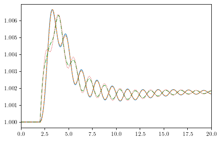
(<Figure size 480x320 with 1 Axes>, <AxesSubplot:>)
Altering Fault duration#
Alter can be used for updating any model parameter. We show another example
of updating the duration of a fault. Using the ieee14_fault.xlsx test case, we have
ss = andes.run(get_case("ieee14/ieee14_fault.xlsx"))
Working directory: "/home/hacui/repos/andes/examples"
> Loaded config from file "/home/hacui/.andes/andes.rc"
> Reloaded generated Python code of module "pycode".
Parsing input file "/home/hacui/repos/andes/andes/cases/ieee14/ieee14_fault.xlsx"...
Input file parsed in 0.0546 seconds.
System internal structure set up in 0.0348 seconds.
-> System connectivity check results:
  No islanded bus detected.
  System is interconnected.
  Each island has a slack bus correctly defined and enabled.

-> Power flow calculation
           Numba: Off
   Sparse solver: KLU
 Solution method: NR method
Power flow initialized in 0.0037 seconds.
0: |F(x)| = 0.5605182134
1: |F(x)| = 0.006202200332
2: |F(x)| = 5.819382824e-06
3: |F(x)| = 6.96508129e-12
Converged in 4 iterations in 0.0047 seconds.
Initialization for dynamics completed in 0.0353 seconds.
Initialization was successful.
Report saved to "ieee14_fault_out.txt" in 0.0021 seconds.
-> Single process finished in 0.3141 seconds.
Again, if you need to add devices, you should use ss = andes.load(.., setup=False) and ss.setup() instead of andes.run().
List the existing Fault devices:
ss.Fault.as_df()
| idx | u | name | bus | tf | tc | xf | rf | |
|---|---|---|---|---|---|---|---|---|
| uid | ||||||||
| 0 | 1 | 1.0 | Fault_1 | 9 | 1.0 | 1.1 | 0.0001 | 0.0 |
One fault on Bus 9 is applied at t=1.0 sec and cleared at t=1.1 sec. Suppose that we want to clear the fault at t = 1.05 sec, we can do
ss.Fault.alter('tc', 1, 1.05) # arguments are `src`, `idx`, `value`
where tc is the parameter to alter, 1 is the idx of the Fault to find, and
1.05 is the new value. Inspect the Fault devices to see the updated value.
The simulation for the new system can be performed next.
ss.Fault.as_df()
| idx | u | name | bus | tf | tc | xf | rf | |
|---|---|---|---|---|---|---|---|---|
| uid | ||||||||
| 0 | 1 | 1.0 | Fault_1 | 9 | 1.0 | 1.05 | 0.0001 | 0.0 |
Cleanup#
!andes misc -C
"/home/hacui/repos/andes/examples/kundur_full_out.txt" removed.
"/home/hacui/repos/andes/examples/kundur_out.lst" removed.
"/home/hacui/repos/andes/examples/kundur_out.npz" removed.
"/home/hacui/repos/andes/examples/ieee14_fault_out.txt" removed.
"/home/hacui/repos/andes/examples/kundur_out.txt" removed.
!rm new_system.xlsx