Changing Setpoints#
This notebook shows an example of changing the generator setpoints in a time-domain simulation. Data in this example is trivial, but the example can be retrofitted for scenarios such as economic dispatch incorporation or reinforcement learning.
Steps are the folllwing:
Initialize a system by running the power flow,
Set the first simulation stop time in
TDS.config.tf,Run the simulation,
Update the setpoints,
Set the new simulation stop time and repeat from 3 until the end.
Step 1: Case Setup#
import andes
from andes.utils import get_case
kundur = get_case('kundur/kundur_full.xlsx')

ss = andes.run(kundur)
Working directory: "/home/hacui/repos/andes/examples"
> Loaded config from file "/home/hacui/.andes/andes.rc"
> Loaded generated Python code in "/home/hacui/.andes/pycode".
Parsing input file "/home/hacui/repos/andes/andes/cases/kundur/kundur_full.xlsx"...
Input file parsed in 0.2635 seconds.
System internal structure set up in 0.0315 seconds.
-> System connectivity check results:
  No islanded bus detected.
  System is interconnected.
  Each island has a slack bus correctly defined and enabled.

-> Power flow calculation
           Numba: Off
   Sparse solver: KLU
 Solution method: NR method
Power flow initialized in 0.0087 seconds.
0: |F(x)| = 14.9282832
1: |F(x)| = 3.608627841
2: |F(x)| = 0.1701107882
3: |F(x)| = 0.002038626956
4: |F(x)| = 3.745104027e-07
Converged in 5 iterations in 0.0108 seconds.
Initialization for dynamics completed in 0.0395 seconds.
Initialization was successful.
Report saved to "kundur_full_out.txt" in 0.0023 seconds.
-> Single process finished in 0.5215 seconds.
# disable the Toggle in this case
ss.Toggle.alter('u', 1, 0)
Step 2: Set the First Stop Time#
# simulate to t=1 sec

# specify the first stop in `ss.TDS.config.tf`
ss.TDS.config.tf = 1
Step 3: Run Simulation#
ss.TDS.run()
-> Time Domain Simulation Summary:
Sparse Solver: KLU
Simulation time: 0.0-1 s.
Fixed step size: h=33.33 ms. Shrink if not converged.
Simulation completed in 0.0245 seconds.
Outputs to "kundur_full_out.lst" and "kundur_full_out.npz".
Outputs written in 0.0039 seconds.
True
Step 4. Apply the auxiliary power setpoints to TGOV1.paux0.v#
First, let's check the equations of TGOV1. ss.TGOV1.paux0 is associated with equation 0 = paux - paux0, in which paux is added to the power input equation.
print(ss.TGOV1.doc())
Model <TGOV1> in Group <TurbineGov>
TGOV1 turbine governor model.

Implements the PSS/E TGOV1 model without deadband.

Parameters

 Name  |            Description            | Default | Unit |    Properties
-------+-----------------------------------+---------+------+-----------------
 idx   | unique device idx                 |         |      |
 u     | connection status                 | 1       | bool |
 name  | device name                       |         |      |
 syn   | Synchronous generator idx         |         |      | mandatory,unique
 Tn    | Turbine power rating. Equal to    |         | MVA  |
       | `Sn` if not provided.             |         |      |
 wref0 | Base speed reference              | 1       | p.u. |
 R     | Speed regulation gain (mach. base | 0.050   | p.u. | ipower
       | default)                          |         |      |
 VMAX  | Maximum valve position            | 1.200   | p.u. | power
 VMIN  | Minimum valve position            | 0       | p.u. | power
 T1    | Valve time constant               | 0.100   |      |
 T2    | Lead-lag lead time constant       | 0.200   |      |
 T3    | Lead-lag lag time constant        | 10      |      |
 Dt    | Turbine damping coefficient       | 0       |      | power
 Sg    | Rated power from generator        | 0       | MVA  |
 ug    | Generator connection status       | 0       | bool |
 Vn    | Rated voltage from generator      | 0       | kV   |

Variables

 Name  |   Type   |             Description              | Unit | Properties
-------+----------+--------------------------------------+------+-----------
 LAG_y | State    | State in lag TF                      |      | v_str
 LL_x  | State    | State in lead-lag                    |      | v_str
 omega | ExtState | Generator speed                      | p.u. |
 paux  | Algeb    | Auxiliary power input                |      | v_str
 pout  | Algeb    | Turbine final output power           |      | v_str
 wref  | Algeb    | Speed reference variable             |      | v_str
 pref  | Algeb    | Reference power input                |      | v_str
 wd    | Algeb    | Generator speed deviation            | p.u. | v_str
 pd    | Algeb    | Pref plus speed deviation times gain | p.u. | v_str
 LL_y  | Algeb    | Output of lead-lag                   |      | v_str
 tm    | ExtAlgeb | Mechanical power interface to SynGen |      |

Initialization Equations

 Name  |   Type   | Initial Value
-------+----------+--------------
 LAG_y | State    | pd * 1 / 1
 LL_x  | State    | LAG_y
 omega | ExtState |
 paux  | Algeb    | paux0
 pout  | Algeb    | ue * tm0
 wref  | Algeb    | wref0
 pref  | Algeb    | tm0 * R
 wd    | Algeb    | 0
 pd    | Algeb    | ue * tm0
 LL_y  | Algeb    | LAG_y
 tm    | ExtAlgeb |

Differential Equations

 Name  |   Type   | RHS of Equation "T x' = f(x, y)" | T (LHS)
-------+----------+----------------------------------+--------
 LAG_y | State    | 1 * pd - 1 * LAG_y               | T1
 LL_x  | State    | (LAG_y - LL_x)                   | T3
 omega | ExtState |                                  |

Algebraic Equations

Name  |   Type   |                RHS of Equation "0 = g(x, y)"
------+----------+------------------------------------------------------------
 paux | Algeb    | paux0 - paux
 pout | Algeb    | ue * (LL_y - Dt * wd) - pout
 wref | Algeb    | wref0 - wref
 pref | Algeb    | pref0 * R - pref
 wd   | Algeb    | ue * (omega - wref) - wd
 pd   | Algeb    | ue*(- wd + pref + paux) * gain - pd
 LL_y | Algeb    | 1 * T2 * (LAG_y - LL_x) + 1 * LL_x * T3 - LL_y * T3+
      |          | LL_LT1_z1 * LL_LT2_z1 * (LL_y - 1 * LL_x)
 tm   | ExtAlgeb | ue * (pout - tm0)

Services

 Name  | Equation |     Type
-------+----------+-------------
 ue    | u * ug   | ConstService
 pref0 | tm0      | ConstService
 paux0 | 0        | ConstService
 gain  | ue/R     | ConstService

Discretes

  Name   |    Type    |      Info
---------+------------+---------------
 LAG_lim | AntiWindup | Limiter in Lag
 LL_LT1  | LessThan   |
 LL_LT2  | LessThan   |

Blocks

Name |     Type      | Info
-----+---------------+-----
 LAG | LagAntiWindup |
 LL  | LeadLag       |


Config Fields in [TGOV1]

   Option     | Value |                Info                | Acceptable values
--------------+-------+------------------------------------+------------------
 allow_adjust | 1     | allow adjusting upper or lower     | (0, 1)
              |       | limits                             |
 adjust_lower | 0     | adjust lower limit                 | (0, 1)
 adjust_upper | 1     | adjust upper limit                 | (0, 1)
ss.TGOV1.paux0.v
array([0., 0., 0., 0.])
# look up the original values of TGOV1 make sure they are as expected

ss.TGOV1.paux0.v
array([0., 0., 0., 0.])
# MUST use in-place assignments.
# Here, we increase the setpoint of the 0-th generator

# method 1: use in-place assignment again

ss.TGOV1.paux0.v[0] = 0.05

# method 2: use ``ss.TGOV1.alter()``

# ss.TGOV1.alter('paux0', 1, 0.05)
ss.TGOV1.paux0.v
array([0.05, 0. , 0. , 0. ])
Continue to simulate to 2 seconds.
ss.TDS.config.tf = 2
ss.TDS.run()
Simulation completed in 0.0916 seconds.
Outputs to "kundur_full_out.lst" and "kundur_full_out.npz".
Outputs written in 0.0032 seconds.
True
ss.TDS.plotter.plot(ss.TGOV1.paux)
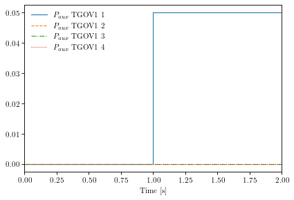
(<Figure size 480x320 with 1 Axes>, <AxesSubplot:xlabel='Time [s]'>)
ss.TDS.plotter.plot(ss.TGOV1.pout)
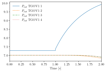
(<Figure size 480x320 with 1 Axes>, <AxesSubplot:xlabel='Time [s]'>)
ss.TDS.plotter.plot(ss.GENROU.omega)
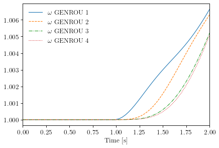
(<Figure size 480x320 with 1 Axes>, <AxesSubplot:xlabel='Time [s]'>)
Step 5: Set Another New Setpoints and New Ending TIme.#
In this example, we clear the auxiliary power previously set to TGOV1.paux0.v
# method 1: use in-place assignment again

ss.TGOV1.paux0.v[0] = 0.

# method 2: use ``ss.TGOV1.alter()``

# ss.TGOV1.alter('paux0', 1, 0)

# set the new ending time to 10 sec.
ss.TDS.config.tf = 10
ss.TDS.run()
Simulation completed in 0.6068 seconds.
Outputs to "kundur_full_out.lst" and "kundur_full_out.npz".
Outputs written in 0.0275 seconds.
True
ss.TDS.plotter.plot(ss.TGOV1.paux)
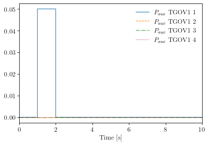
(<Figure size 480x320 with 1 Axes>, <AxesSubplot:xlabel='Time [s]'>)
ss.TDS.plotter.plot(ss.GENROU.omega)
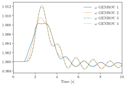
(<Figure size 480x320 with 1 Axes>, <AxesSubplot:xlabel='Time [s]'>)
!andes misc -C
"/home/hacui/repos/andes/examples/kundur_full_out.npz" removed.
"/home/hacui/repos/andes/examples/kundur_full_out.txt" removed.
"/home/hacui/repos/andes/examples/kundur_full_out.lst" removed.