MATPOWER Interface#
See also the API reference for andes.interop.matpower.
import andes

from andes.interop.matpower import (start_instance,
    to_matpower, from_matpower)
Create an Octave/MATLAB instance#
m = start_instance()
Convert to MATPOWER#
ss = andes.system.example()  # load an ieee14 example case

mpc = to_matpower(m, 'mpc', ss)
Test if the power flow of mpc can be solved
m.eval("runpf(mpc)")
warning: error caught while executing handle class delete method:
'osqp_mex' undefined near line 40 column 13
OSQP Error!

MATPOWER Version 7.1, 08-Oct-2020 -- AC Power Flow (Newton)

Newton's method power flow (power balance, polar) converged in 3 iterations.

Converged in 0.01 seconds
================================================================================
|     System Summary                                                           |
================================================================================

How many?                How much?              P (MW)            Q (MVAr)
---------------------    -------------------  -------------  -----------------
Buses             14     Total Gen Capacity     400.0        -112.0 to 150.0
Generators         5     On-line Capacity       400.0        -112.0 to 150.0
Committed Gens     5     Generation (actual)    226.4              49.8
Loads             11     Load                   223.7              95.4
  Fixed           11       Fixed                223.7              95.4
  Dispatchable     0       Dispatchable          -0.0 of -0.0      -0.0
Shunts             2     Shunt (inj)             -0.0              35.3
Branches          20     Losses (I^2 * Z)         2.73             13.52
Transformers      20     Branch Charging (inj)     -               23.8
Inter-ties         0     Total Inter-tie Flow     0.0               0.0
Areas              1

                          Minimum                      Maximum
                 -------------------------  --------------------------------
Voltage Magnitude   1.010 p.u. @ bus 3          1.030 p.u. @ bus 2
Voltage Angle      -9.48 deg   @ bus 14         0.00 deg   @ bus 1
P Losses (I^2*R)             -                  0.50 MW    @ line 1-2
Q Losses (I^2*X)             -                  2.11 MVAr  @ line 8-7

================================================================================
|     Bus Data                                                                 |
================================================================================
 Bus      Voltage          Generation             Load
  #   Mag(pu) Ang(deg)   P (MW)   Q (MVAr)   P (MW)   Q (MVAr)
----- ------- --------  --------  --------  --------  --------
    1  1.030    0.000*    81.43    -21.62       -         -
    2  1.030   -1.764     40.00     30.44     21.70     12.70
    3  1.010   -3.537     40.00     12.60     50.00     25.00
    4  1.011   -4.410       -         -       47.80     10.00
    5  1.017   -3.843       -         -        7.60      1.60
    6  1.030   -6.453     30.00     20.99     15.00      7.50
    7  1.022   -4.885       -         -         -         -
    8  1.030   -1.540     35.00      7.40       -         -
    9  1.022   -7.246       -         -       29.50     16.60
   10  1.016   -7.415       -         -        9.00      5.80
   11  1.019   -7.080       -         -        3.50      1.80
   12  1.017   -7.473       -         -        6.10      1.60
   13  1.014   -7.721       -         -       13.50      5.80
   14  1.016   -9.481       -         -       20.00      7.00
                        --------  --------  --------  --------
               Total:    226.43     49.80    223.70     95.40

================================================================================
|     Branch Data                                                              |
================================================================================
Brnch   From   To    From Bus Injection   To Bus Injection     Loss (I^2 * Z)
  #     Bus    Bus    P (MW)   Q (MVAr)   P (MW)   Q (MVAr)   P (MW)   Q (MVAr)
-----  -----  -----  --------  --------  --------  --------  --------  --------
   1      1      2     50.10    -18.36    -49.60     14.29     0.503      1.53
   2      1      5     31.33     -3.26    -30.83      0.17     0.500      2.06
   3      2      3     17.79      4.11    -17.63     -8.00     0.158      0.67
   4      2      4     28.02      0.46    -27.58     -2.69     0.433      1.31
   5      2      5     22.09     -1.13    -21.83     -1.70     0.262      0.80
   6      3      4      7.63     -4.40     -7.58      3.21     0.047      0.12
   7      4      5    -25.97     -5.70     26.07      5.99     0.092      0.29
   8      6     11      6.91      2.37     -6.86     -2.27     0.048      0.10
   9      6     12      7.93      1.32     -7.86     -1.17     0.075      0.16
  10      6     13     19.15      2.76    -18.92     -2.31     0.234      0.46
  11      7      9     39.12      1.46    -39.12      0.15     0.000      1.61
  12      9     10      5.67      5.40     -5.65     -5.35     0.019      0.05
  13      9     14     13.17     -3.85    -12.94      4.34     0.229      0.49
  14     10     11     -3.35     -0.45      3.36      0.47     0.009      0.02
  15     12     13      1.76     -0.43     -1.75      0.44     0.007      0.01
  16     13     14      7.17     -3.93     -7.06      4.16     0.111      0.23
  17      4      7      4.12     -3.76     -4.12      3.83    -0.000      0.06
  18      4      9      9.22     -1.06     -9.22      1.53     0.000      0.47
  19      6      5    -18.99      7.03     18.99     -6.06     0.000      0.97
  20      8      7     35.00      7.40    -35.00     -5.29     0.000      2.11
                                                             --------  --------
                                                    Total:     2.727     13.52
mpc_sol = m.pull("mpc") # retrieve the solution
One can also save the case to a MATPOWER .m file from Octave/MATLAB. Comment
in and run the following code:
# m.eval("savecase('case14_andes.m', mpc)")
Convert from MATPOWER#
system = from_matpower(m, 'mpc')
m.pull() won't work if one has run OPF in Octave/MATLAB because Oct2Py does not support custom class objects created by MATPOWER.
from _matpower() will read the individual fields to construct an mpc dict internally before creating a system.
Add dynamic data#
One can create an Excel file with dynamic data only and use the xlsx parser to load data into system:
from andes.io import xlsx

xlsx.read(system, andes.get_case('ieee14/ieee14_dyn_only.xlsx'))
<andes.system.System at 0x7f8684043520>
system.setup()

system.PFlow.run()

system.TDS.run()
<Fault 1>: Applying fault on Bus (idx=7) at t=1.0 sec.
<Fault 1>: Clearing fault on Bus (idx=7) at t=1.03333 sec.
True
system.TDS.plt.plot(system.GENROU.omega)
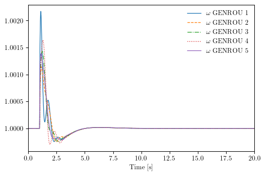
(<Figure size 600x400 with 1 Axes>, <AxesSubplot:xlabel='Time [s]'>)
Since the data in ieee14_dyn_only.xlsx is stripped from ieee14/ieee14_fault.xlsx, the above results is identical to the simulation of the latter case:
ss = andes.run(andes.get_case("ieee14/ieee14_fault.xlsx"),
               routine='tds', verbose=30,
               no_output=True, default_config=True)
<Fault 1>: Applying fault on Bus (idx=9) at t=1.0 sec.
<Fault 1>: Clearing fault on Bus (idx=9) at t=1.1 sec.
-> Single process finished in 0.7220 seconds.
ss.TDS.plt.plot(ss.GENROU.omega)
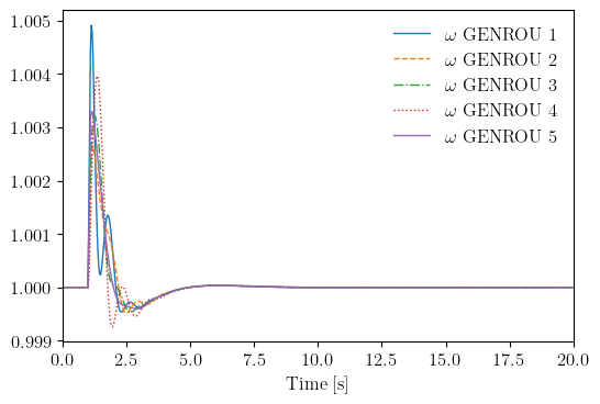
(<Figure size 600x400 with 1 Axes>, <AxesSubplot:xlabel='Time [s]'>)