pandapower Interface

This example (1) shows how to convert an ANDES system (ssa) to a pandapower network (ssp), (2) benchmarks the powerflow results, (3) shows how to alter ssa active power setpoints according to ssp results.

The following clarafications you might need to know:

1. This interface tracks static power flow model in ANDES: Bus, Line, PQ, Shunt, PV, and Slack. The dynamic model in ANDES is not tracked, including but not limited to TurbineGov, SynGen, and Exciter.

2. The interface converts the Slack in ANDES to gen in pandapower rather than ext_gen.

3. MUST NOT verify power flow after initializing TDS in ANDES. ANDES does not allow running PFlow for systems with initialized TDS as it will break variable addressing.

4. If you want to track dynamic model outputs in ANDES and feedback into pandapower, you might need to manually transfer the results from ANDES to pandapower.

This interface is mainly developed by Jinning Wang.

import andes

from andes.interop.pandapower import to_pandapower, \
    make_link_table, runopp_map, add_gencost

andes.config_logger(20)

import pandapower as pp
import numpy as np
import pandas as pd

from math import pi

Load case

Here we use the same ANDES system ss0 to do the pandapower conversion, which leaves the ssa untouched.

This will be useful if you need to modify the ssa parametes or setpoints.

ssa = andes.load(andes.get_case('ieee14/ieee14_ieeet1.xlsx'),
                 setup=False,
                 no_output=True,
                 default_config=True)
ssa.Toggle.u.v = [0, 0]
ssa.setup()

ss0 = andes.load(andes.get_case('ieee14/ieee14_ieeet1.xlsx'),
                 setup=False,
                 no_output=True,
                 default_config=True)
ss0.Toggle.u.v = [0, 0]
ss0.setup()

Working directory: "/Users/jinningwang/Documents/work/andes/docs/source/examples"
> Loaded generated Python code in "/Users/jinningwang/.andes/pycode".
Generated code for <PQ> is stale.
Numerical code generation (rapid incremental mode) started...

Generating code for 1 models on 8 processes.

Saved generated pycode to "/Users/jinningwang/.andes/pycode"
> Reloaded generated Python code of module "pycode".
Generated numerical code for 1 models in 0.1328 seconds.
Parsing input file "/Users/jinningwang/Documents/work/andes/andes/cases/ieee14/ieee14_ieeet1.xlsx"...
Input file parsed in 0.0441 seconds.
System internal structure set up in 0.0236 seconds.
Working directory: "/Users/jinningwang/Documents/work/andes/docs/source/examples"
> Reloaded generated Python code of module "pycode".
Generated code for <PQ> is stale.
Numerical code generation (rapid incremental mode) started...

Generating code for 1 models on 8 processes.

Saved generated pycode to "/Users/jinningwang/.andes/pycode"
> Reloaded generated Python code of module "pycode".
Generated numerical code for 1 models in 0.2553 seconds.
Parsing input file "/Users/jinningwang/Documents/work/andes/andes/cases/ieee14/ieee14_ieeet1.xlsx"...
Input file parsed in 0.0367 seconds.
System internal structure set up in 0.0227 seconds.

True

Convert to pandapower net

Convert ADNES system ssa to pandapower net ssp.

ssp = to_pandapower(ss0)

-> System connectivity check results:
  No islanded bus detected.
  System is interconnected.
  Each island has a slack bus correctly defined and enabled.

-> Power flow calculation
           Numba: Off
   Sparse solver: KLU
 Solution method: NR method
Power flow initialized in 0.0029 seconds.
0: |F(x)| = 0.5605182134
1: |F(x)| = 0.006202200332
2: |F(x)| = 5.819382825e-06
3: |F(x)| = 6.957087684e-12
Converged in 4 iterations in 0.0038 seconds.
Power flow results are consistent. Conversion is successful.

Add generator cost data.

gen_cost = np.array([
        [2, 0, 0, 3, 0.0430293, 20, 0], 
        [2, 0, 0, 3, 0.25,      20, 0], 
        [2, 0, 0, 3, 0.01,      40, 0], 
        [2, 0, 0, 3, 0.01,      40, 0], 
        [2, 0, 0, 3, 0.01,      40, 0]
])

add_gencost(ssp, gen_cost)

True

Inspect the pandapower net ssp.

ssp

This pandapower network includes the following parameter tables:
   - bus (14 elements)
   - load (11 elements)
   - gen (5 elements)
   - shunt (2 elements)
   - line (16 elements)
   - trafo (4 elements)
   - poly_cost (5 elements)
 and the following results tables:
   - res_bus (14 elements)
   - res_line (16 elements)
   - res_trafo (4 elements)
   - res_load (11 elements)
   - res_shunt (2 elements)
   - res_gen (5 elements)

Comapre Power Flow Results

Run power flow of ssa.

ssa.PFlow.run()

-> System connectivity check results:
  No islanded bus detected.
  System is interconnected.
  Each island has a slack bus correctly defined and enabled.

-> Power flow calculation
           Numba: Off
   Sparse solver: KLU
 Solution method: NR method
Power flow initialized in 0.0039 seconds.
0: |F(x)| = 0.5605182134
1: |F(x)| = 0.006202200332
2: |F(x)| = 5.819382825e-06
3: |F(x)| = 6.957087684e-12
Converged in 4 iterations in 0.0045 seconds.

True

# ssa
ssa_res_gen = pd.DataFrame(columns=['name', 'p_mw', 'q_mvar', 'va_degree', 'vm_pu'])
ssa_res_gen['name'] = ssa.PV.as_df()['name']
ssa_res_gen['p_mw'] = ssa.PV.p.v * ssa.config.mva
ssa_res_gen['q_mvar'] = ssa.PV.q.v * ssa.config.mva
ssa_res_gen['va_degree'] = ssa.PV.a.v * 180 / pi
ssa_res_gen['vm_pu'] = ssa.PV.v.v
ssa_res_slack = pd.DataFrame([[ssa.Slack.name.v[0], ssa.Slack.p.v[0] * ssa.config.mva,
                              ssa.Slack.q.v[0] * ssa.config.mva, ssa.Slack.a.v[0] * 180 / pi,
                              ssa.Slack.v.v[0]]],
                             columns=ssa_res_gen.columns,
                             )
ssa_res_gen = pd.concat([ssa_res_gen, ssa_res_slack]).reset_index(drop=True)

# ssp
pp.runpp(ssp)
ssp_res_gen = pd.concat([ssp.gen['name'], ssp.res_gen], axis=1)

res_gen_concat = pd.concat([ssa_res_gen, ssp_res_gen], axis=1)

# ssa
ssa_pf_bus = ssa.Bus.as_df()[["name"]].copy()
ssa_pf_bus['v_andes'] = ssa.Bus.v.v
ssa_pf_bus['a_andes'] = ssa.Bus.a.v * 180 / pi

# ssp
ssp_pf_bus = ssa.Bus.as_df()[["name"]].copy()
ssp_pf_bus['v_pp'] = ssp.res_bus['vm_pu']
ssp_pf_bus['a_pp'] = ssp.res_bus['va_degree']

pf_bus_concat = pd.concat([ssa_pf_bus, ssp_pf_bus], axis=1)

Generation

In the table below, the left half are ANDES results, and the right half are from pandapower

res_gen_concat.round(4)

	name	p_mw	q_mvar	va_degree	vm_pu	name	p_mw	q_mvar	va_degree	vm_pu
0	2	40.0000	30.4361	-1.7641	1.03	2	40.0000	30.4361	-1.7641	1.03
1	3	40.0000	12.5971	-3.5371	1.01	3	40.0000	12.5971	-3.5371	1.01
2	4	30.0000	20.9866	-6.4527	1.03	4	30.0000	20.9866	-6.4527	1.03
3	5	35.0000	7.3964	-1.5400	1.03	5	35.0000	7.3964	-1.5400	1.03
4	1	81.4272	-21.6171	0.0000	1.03	1	81.4272	-21.6171	0.0000	1.03

Bus voltage and angle

Likewise, the left half are ANDES results, and the right half are from pandapower

pf_bus_concat.round(4)

	name	v_andes	a_andes	name	v_pp	a_pp
uid
0	BUS1	1.0300	0.0000	BUS1	1.0300	0.0000
1	BUS2	1.0300	-1.7641	BUS2	1.0300	-1.7641
2	BUS3	1.0100	-3.5371	BUS3	1.0100	-3.5371
3	BUS4	1.0114	-4.4098	BUS4	1.0114	-4.4098
4	BUS5	1.0173	-3.8430	BUS5	1.0173	-3.8430
5	BUS6	1.0300	-6.4527	BUS6	1.0300	-6.4527
6	BUS7	1.0225	-4.8852	BUS7	1.0225	-4.8852
7	BUS8	1.0300	-1.5400	BUS8	1.0300	-1.5400
8	BUS9	1.0218	-7.2459	BUS9	1.0218	-7.2459
9	BUS10	1.0155	-7.4155	BUS10	1.0155	-7.4155
10	BUS11	1.0191	-7.0797	BUS11	1.0191	-7.0797
11	BUS12	1.0174	-7.4730	BUS12	1.0174	-7.4730
12	BUS13	1.0145	-7.7208	BUS13	1.0145	-7.7208
13	BUS14	1.0163	-9.4811	BUS14	1.0163	-9.4811

Generator dispatch based on OPF from pandapower

Prepare the link table.

# Asign the StaticGen with OPF, in this case, all the SynGen are GENROU
link_table = make_link_table(ssa)

link_table

	stg_name	stg_u	stg_idx	bus_idx	dg_idx	rg_idx	rexc_idx	syg_idx	exc_idx	gov_idx	bus_name	gammap	gammaq
0	1	1.0	1	1	NaN	NaN	NaN	GENROU_1	ESST3A_2	TGOV1_1	BUS1	1.0	1.0
1	2	1.0	2	2	NaN	NaN	NaN	GENROU_2	EXST1_1	TGOV1_2	BUS2	1.0	1.0
2	3	1.0	3	3	NaN	NaN	NaN	GENROU_3	ESST3A_3	TGOV1_3	BUS3	1.0	1.0
3	4	1.0	4	6	NaN	NaN	NaN	GENROU_4	ESST3A_4	TGOV1_4	BUS6	1.0	1.0
4	5	1.0	5	8	NaN	NaN	NaN	GENROU_5	1	TGOV1_5	BUS8	1.0	1.0

Note: some Jupyter notebooks may not support inline plots. You can use the following command to enable it.

import matplotlib
%matplotlib inline

import matplotlib
%matplotlib inline

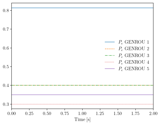
Run the TDS in ADNES to 2s.

ssa.TDS.config.tf = 2
ssa.TDS.run()

ssa.TDS.plt.plot(ssa.GENROU.Pe)

-> Time Domain Simulation Summary:
Sparse Solver: KLU
Simulation time: 0.0-2 s.
Fixed step size: h=33.33 ms. Shrink if not converged.
Initialization for dynamics completed in 0.1282 seconds.
Initialization was successful.

Simulation to t=2.00 sec completed in 0.0623 seconds.

(<Figure size 640x480 with 1 Axes>, <AxesSubplot:xlabel='Time [s]'>)

Get the OPF results from pandapower. The ssp_res has been converted to p.u..

ssp_res = runopp_map(ssp, link_table)
ssp_res

ACOPF is solved.

	stg_idx	p	q	vm_pu	bus_idx	controllable	dg_idx	rg_idx	syg_idx	gov_idx	exc_idx
0	2	0.5	0.129107	1.096903	2	True	NaN	NaN	GENROU_2	TGOV1_2	EXST1_1
1	3	0.41275	0.149997	1.082551	3	True	NaN	NaN	GENROU_3	TGOV1_3	ESST3A_3
2	4	0.34426	0.099998	1.086084	6	True	NaN	NaN	GENROU_4	TGOV1_4	ESST3A_4
3	5	0.495878	0.085204	1.099996	8	True	NaN	NaN	GENROU_5	TGOV1_5	1
4	1	0.5	-0.079016	1.100000	1	True	NaN	NaN	GENROU_1	TGOV1_1	ESST3A_2

Now dispatch the resutls into ssa, where the active power setpoitns are updated to TurbinGov.pref0.

ssa_gov_idx = list(ssp_res['gov_idx'][~ssp_res['gov_idx'].isna()])
ssa.TurbineGov.set(src='pref0', idx=ssa_gov_idx, attr='v', value=ssp_res['p'][~ssp_res['gov_idx'].isna()])
ssa.TurbineGov.get(src='pref0', idx=ssa_gov_idx, attr='v')

array([0.49999998, 0.41274963, 0.34426   , 0.49587786, 0.50000031])

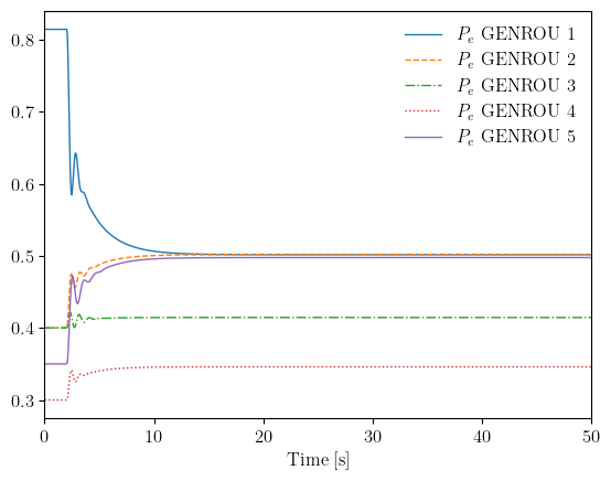
Now run the TDS to 50s.

ssa.TDS.config.tf = 50
ssa.TDS.run()

Simulation to t=50.00 sec completed in 1.9001 seconds.

True

We can see the outputs of GENROU are rearranged by the OPF results.

ssa.TDS.plt.plot(ssa.GENROU.Pe)

(<Figure size 640x480 with 1 Axes>, <AxesSubplot:xlabel='Time [s]'>)