Simulate and Plot#
Import and Setting the Verbosity Level#
We first import the andes library and the get_case function that for loading test cases shipped with ANDES.
import andes

from andes.utils.paths import get_case
We can configure the verbosity level for logging (output messages) by passing a verbosity level (10-DEBUG, 20-INFO, 30-WARNING, 40-ERROR, 50-CRITICAL) to the stream_level argument of andes.main.config_logger(). Verbose level 10 is useful for getting debug output.
The logging level can be altered (as of v1.4.3) by calling config_logger again with new stream_level and file_level.
andes.config_logger(stream_level=20)
Note that the above andes.config_logger() is a shorthand to andes.main.config_logger().
If this step is omitted, the default INFO level (stream_level=20) will be used.
Run Time-Domain Simulation#
Run power flow by default#
get_case takes a relative path to ANDES_ROOT/andes/cases and returns the full path, where ANDES_ROOT is the root folder of ANDES.
andes.run is the entrypoint function for loading files and running routines. It runs power flow by default and returns a System object.
Note: if default_config=True, the default concif will be used. To use your own config, remove default_config=True.
See the tutorial for saving and editing ANDES config.
ss = andes.run(get_case('kundur/kundur_full.xlsx'), default_config=True)
Working directory: "/home/hacui/repos/andes/examples"
> Loaded generated Python code in "/home/hacui/.andes/pycode".
Parsing input file "/home/hacui/repos/andes/andes/cases/kundur/kundur_full.xlsx"...
Input file parsed in 0.2775 seconds.
System internal structure set up in 0.0322 seconds.
-> System connectivity check results:
  No islanded bus detected.
  System is interconnected.
  Each island has a slack bus correctly defined and enabled.

-> Power flow calculation
           Numba: Off
   Sparse solver: KLU
 Solution method: NR method
Power flow initialized in 0.0039 seconds.
0: |F(x)| = 14.9282832
1: |F(x)| = 3.608627841
2: |F(x)| = 0.1701107882
3: |F(x)| = 0.002038626956
4: |F(x)| = 3.745104027e-07
Converged in 5 iterations in 0.0084 seconds.
Report saved to "kundur_full_out.txt" in 0.0020 seconds.
-> Single process finished in 0.5018 seconds.
Run time-domain simulation#
Run TDS by calling TDS.run() on the system. Note that the call must follow the power flow immediately.
The default simulation is for 20 seconds. To change if, change config.tf to the desired value.
ss.TDS.config.tf = 10 # simulate for 10 seconds
ss.TDS.run()
-> Time Domain Simulation Summary:
Sparse Solver: KLU
Simulation time: 0.0-10 s.
Fixed step size: h=33.33 ms. Shrink if not converged.
Initialization for dynamics completed in 0.0490 seconds.
Initialization was successful.
<Toggle 1>: Line.Line_8 status changed to 0 at t=2.0 sec.
Simulation completed in 0.5985 seconds.
Outputs to "kundur_full_out.lst" and "kundur_full_out.npz".
Outputs written in 0.0104 seconds.
True
To check if all operations completed successfully, check ss.exit_code. exit_code == 0 means that all operations were successful.
If not zero, exit_code indicates the number of errors caught. One will need to check output messages for errors.
ss.exit_code
0
Export and Plot Results#
If you are using ANDES interactively from Jupyter Notebook or IPython, at the end of a time-domain simulation. a plotter object ss.TDS.plt will automatically be created.
To check if that has been created successfully (in case the detection of an interactive environment fails), check the type of ss.TDS.plt.
ss.TDS.plt
<andes.plot.TDSData at 0x7fb229d9ff70>
If ss.TDS.plt is None, it can be manually loaded with ss.TDS.load_plotter(). Otherwise, load_plotter() can be safely skipped.
ss.TDS.load_plotter()
Exporting simulation data to csv#
To export simulation results to a CSV file, one can use ss.TDS.plt.export_csv(), which takes an optional argument of the file name.
If not provided, a default file name will be assigned.
ss.TDS.plt.export_csv()
CSV data saved to "/home/hacui/repos/andes/examples/kundur_full_out.csv".
Index-based Plotting#
plotter.plot() is the entry point for plotting. It is the backend of the command-line andes plot.
Before plotting, open the kundur_full_out.lst to find the indices (first column) for the variables to plot.
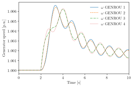
For example, if we want to plot all generator speed, which is the omega variable of GENROU.
By inspect, we found the indices as 5, 6, 7, 8.
Pass them in a tuple or a list to ss.TDS.plt.plot.
fig, ax = ss.TDS.plt.plot((5, 6, 7, 8))
plot() returns a figure object and an axis object.
Find index by variable name#
plotter.find() is a method for finding indices based on variable name.
The first argument is the pattern to find. An optional argument exclude is the pattern to exclude. Regular expression is supported for both.
ss.TDS.plt.find('omega')
([5, 6, 7, 8],
 ['omega GENROU 1', 'omega GENROU 2', 'omega GENROU 3', 'omega GENROU 4'])
fig, ax = ss.TDS.plotter.plot(ss.TDS.plotter.find('omega')[0])

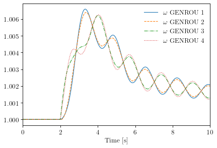
Plotting by variable#
Looking up indices from the lst file can be tedious.
Instead, one can pass a a variable in a model to ss.TDS.plt.plot. For example, to plot ss.GENROU.omega, do
fig, ax = ss.TDS.plt.plot(ss.GENROU.omega)
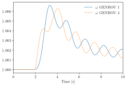
To plot a subset of the variables, pass the 0-indexed selection indices in a tuple through argument a of ss.TDS.plt.plot. For example, to plot the 0-th and the 3-th GENROU.omega, do
fig, ax = ss.TDS.plt.plot(ss.GENROU.omega, a=(0, 3))
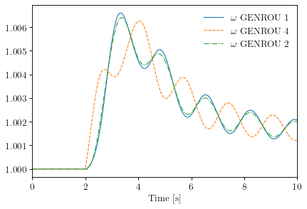
Adding curves to an existing figure#
Plotting curves into an existing figure allows easy comparison of results. It can be done by passing a figure and an axis object of plot().
For example, to plot the speed of the second generator (a=1) on the figure above, do
fig, ax = ss.TDS.plt.plot(ss.GENROU.omega, a=(1, ), fig=fig, ax=ax, linestyles=['-.'])
fig
<Figure size 432x288 with 0 Axes>
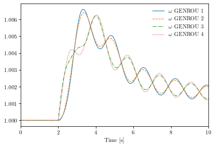
Y-axis label#
fig, ax = ss.TDS.plotter.plot((5, 6, 7, 8), ylabel='Generator speed [p.u.]')
Legend names (yheader)#
fig, ax = ss.TDS.plotter.plot((5, 6, 7, 8), ylabel='Generator speed [p.u.]',
                              yheader=['Spd 1', 'Spd 2', 'Spd 3', 'Spd 4'])
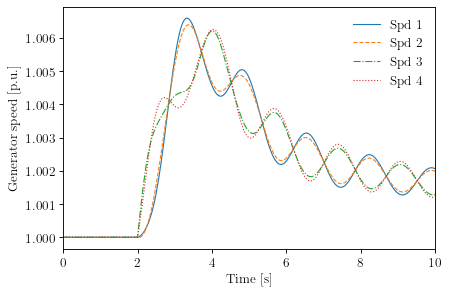
Note that the number of elements passed to yheader should match the number of variables.
yheader only applies to new curves and cannot be used to modify existing legends.
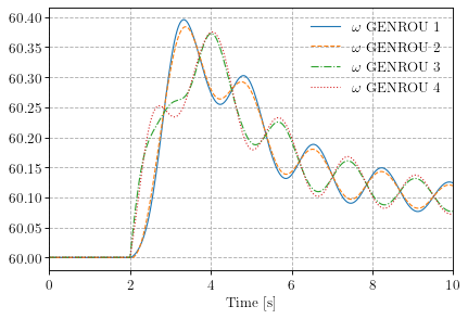
Scaling#
A lambda functino can be passed to ycalc to scale the value. To scale the frequency from per unit to 60 Hz nominal values, use
fig, ax = ss.TDS.plotter.plot((5, 6, 7, 8), ycalc=lambda x: 60 * x)

Greyscale and Grid#
fig, ax = ss.TDS.plotter.plot((5, 6, 7, 8),
                              ycalc=lambda x: 60 * x,
                              greyscale=True,
                              grid=True)
Save figure#
Pass savefig = True to save the figure to a png file.
fig, ax = ss.TDS.plotter.plot((5, 6, 7, 8), savefig=True)
Figure saved to "kundur_full_out_1.png".

Additional arguments#
plotter.plot takes addition arguments. To check additional arguments, please use help or refer to the source code.
help(ss.TDS.plotter.plot)
Help on method plot in module andes.plot:

plot(yidx, xidx=(0,), *, a=None, ytimes=None, ycalc=None, left=None, right=None, ymin=None, ymax=None, xlabel=None, ylabel=None, xheader=None, yheader=None, legend=None, grid=False, greyscale=False, latex=True, dpi=80, line_width=1.0, font_size=12, savefig=None, save_format=None, show=True, title=None, linestyles=None, use_bqplot=False, hline1=None, hline2=None, vline1=None, vline2=None, hline=None, vline=None, fig=None, ax=None, backend=None, set_xlim=True, set_ylim=True, autoscale=False, legend_bbox=None, legend_loc=None, legend_ncol=1, figsize=None, color=None, **kwargs) method of andes.plot.TDSData instance
    Entry function for plotting.

    This function retrieves the x and y values based on the `xidx` and
    `yidx` inputs, applies scaling functions `ytimes` and `ycalc` sequentially,
    and delegates the plotting to the backend.

    Parameters
    ----------
    yidx : list or int
        The indices for the y-axis variables
    xidx : tuple or int, optional
        The index for the x-axis variable
    a : tuple or list, optional
        The 0-indexed sub-indices into `yidx` to plot.
    ytimes : float, optional
        A scaling factor to apply to all y values.
    left : float
        The starting value of the x axis
    right : float
        The ending value of the x axis
    ymin : float
        The minimum value of the y axis
    ymax : float
        The maximum value of the y axis
    ylabel : str
        Text label for the y axis
    yheader : list
        A list containing the variable names for the y-axis variable
    title : str
        Title string to be shown at the top
    fig
        Existing figure object to draw the axis on.
    ax
        Existing axis object to draw the lines on.

    Other Parameters
    ----------------
    ycalc: callable, optional
        A callable to apply to all y values after scaling with `ytimes`.
    xlabel : str
        Text label for the x axis
    xheader : list
        A list containing the variable names for the x-axis variable
    legend : bool
        True to show legend and False otherwise
    legend_ncol : int
        Number of columns in legend
    legend_bbox : tuple of two floats
        legend box to anchor
    grid : bool
        True to show grid and False otherwise
    latex : bool
        True to enable latex and False to disable
    greyscale : bool
        True to use greyscale, False otherwise
    savefig : bool or str
        True to save to png figure file.
        str is treated as the output file name.
    save_format : str
        File extension string (pdf, png or jpg) for the savefig format
    dpi : int
        Dots per inch for screen print or save.
        `savefig` uses a minimum of 200 dpi
    line_width : float
        Plot line width
    font_size : float
        Text font size (labels and legends)
    figsize : tuple
        Figure size passed when creating new figure
    show : bool
        True to show the image
    backend : str or None
        `bqplot` to use the bqplot backend in notebook.
        None for matplotlib.
    hline1: float, optional
        Dashed horizontal line 1
    hline2: float, optional
        Dashed horizontal line 2
    vline1: float, optional
        Dashed horizontal line 1
    vline2: float, optional
        Dashed vertical line 2
    hline: float or Iterable
        y-axis location of horizontal line(s)
    vline: float or Iterable
        x-axis location of vertical line(s)

    Returns
    -------
    (fig, ax)
        Figure and axis handles for matplotlib backend.
    fig
        Figure object for bqplot backend.
Cleanup#
! andes misc -C
"/home/hacui/repos/andes/examples/kundur_full_out.npz" removed.
"/home/hacui/repos/andes/examples/kundur_full_out.txt" removed.
"/home/hacui/repos/andes/examples/kundur_full_out.lst" removed.
"/home/hacui/repos/andes/examples/kundur_full_out.csv" removed.
!rm kundur_full_out_1.png