Batch Processing - in Memory#

This notebook shows examples for batch power flow and time-domain calculations. Readers are supposed to have read the previous examples, especially Example 7 for parallel simulations.

import andes
import numpy as np

from matplotlib import pyplot as plt

Batch Power Flow Calculation#

Use the Kundur's system as the example. Suppose we want to calculate power flow for the same system structure but for different load levels.

kundur = andes.utils.get_case('kundur/kundur_full.xlsx')

ss = andes.run(kundur,
               no_output=True,
               default_config=True,
               verbose=30,  # set logging level to WARNING
               )

-> Single process finished in 0.4701 seconds.

There are two PQ loads in the Kundur's system with idxes of PQ_0 and PQ_1.

ss.PQ.as_df(vin=True)

	idx	u	name	bus	Vn	p0	q0	vmax	vmin	owner
uid
0	PQ_0	1.0	PQ_0	7	230.0	11.59	-0.735	1.1	0.9	1
1	PQ_1	1.0	PQ_1	8	230.0	15.75	-0.899	1.1	0.9	1

If we have a range of active power for each load, such as

n_samples = 3  # Note: increase `n_samples` for higher data resolution 

pq0_values = np.linspace(10, 12, n_samples)
pq1_values = np.linspace(12, 18, n_samples)

where there are 3 samples for PQ_0.p0 between [10, 12] and 3 samples for PQ_1.p0 between (12, 18).

We can use a for loop to set the load values and calculate power flow for each point.

Suppose we want to retrieve the voltage magnitude for each case, we use v_results the voltage results. Results that are not saved will be discarded.

v_results = np.zeros((ss.Bus.n, n_samples ** 2))
idx = 0

for ii in pq0_values:
    ss.PQ.alter("p0", "PQ_0", ii)
    for jj in pq1_values:
        
        ss.PQ.alter("p0", "PQ_1", jj)

        ss.PFlow.run()
        v_results[:, idx] = ss.dae.y[ss.Bus.v.a]
        
        idx += 1

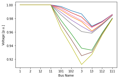
Let's plot the results.

lines = plt.plot(v_results)

xl = plt.xlabel('Bus Name')
yl = plt.ylabel('Voltage [p.u.]')

tk = plt.xticks(np.arange(ss.Bus.n), ss.Bus.name.v)

One should be aware that the for-loop based approach is single-threaded. It does not take advantage of multi-core processors.

If the total number of scenarios are huge, one should refer to Example 7 to save all scenarios to excel files and use multi-processing.

Batch Time-Domain Simulation#

The next example shows how to run batch time-domain simulations for different events.

Suppose we want to create one scenario for each line trip event, which is actuated through Toggle. For the same system, we want to add Toggles for each line, run the simulation, and save results.

kundur = andes.utils.get_case('kundur/kundur_full.xlsx')

We use andes.load() with setup=False to load the test case.

It is important to note that one must pass setup=False so that adding Toggles can be allowed.

ss = andes.load(kundur, setup=False)

The idxes of all available lines to trip are in ss.Line.idx.v:

idxes = ss.Line.idx.v

ss.Toggle.as_df()

	idx	u	name	model	dev	t
uid
0	1	1	Toggle_1	Line	Line_8	2

We use ss.add() to add two Toggles for each line at 1 second and 1.1 seconds to simulate a line opening and closing. ss.add() takes a model name, "Toggle", as the positional argument, and a dictionary for the Toggle device parameters.

A note for this particular test case is that kundur_full.xlsx already comes with a Toggle with idx==1. To not to interfere with our scenarios, we need to disable it using ss.Toggle.alter.

After adding Toggle devices, we need to manually call ss.setup() to finish the data structure setup. Then, power flow and time-domain simulation can be performed.

We store the results in a dictionary where keys are the line names and values are the systems. Code is as follows.

results = dict()

for idx in idxes:
    ss = andes.load(kundur, setup=False)
    
    ss.add('Toggle', dict(model="Line", dev=idx, t=1.0))
    ss.add('Toggle', dict(model="Line", dev=idx, t=1.1))
    
    ss.setup()                     # no `ss.add()` calls are allowed after setup()
    ss.Toggle.alter('u', 1, 0.0)  # disable the existing Toggle with idx=1 (this is for the particular case)

    ss.PFlow.run()
    ss.TDS.config.tf = 5       # simulate for 5 seconds to save time
    ss.TDS.config.no_tqdm = 1  # disable progres bar printing 
    ss.TDS.run()
    
    results[idx] = ss

<Toggle Toggle_2>: Line.Line_0 status changed to 0 at t=1.0 sec.
<Toggle Toggle_3>: Line.Line_0 status changed to 1 at t=1.1 sec.
<Toggle Toggle_2>: Line.Line_1 status changed to 0 at t=1.0 sec.
<Toggle Toggle_3>: Line.Line_1 status changed to 1 at t=1.1 sec.
<Toggle Toggle_2>: Line.Line_2 status changed to 0 at t=1.0 sec.
<Toggle Toggle_3>: Line.Line_2 status changed to 1 at t=1.1 sec.
<Toggle Toggle_2>: Line.Line_3 status changed to 0 at t=1.0 sec.
<Toggle Toggle_3>: Line.Line_3 status changed to 1 at t=1.1 sec.
<Toggle Toggle_2>: Line.Line_4 status changed to 0 at t=1.0 sec.
<Toggle Toggle_3>: Line.Line_4 status changed to 1 at t=1.1 sec.
<Toggle Toggle_2>: Line.Line_5 status changed to 0 at t=1.0 sec.
<Toggle Toggle_3>: Line.Line_5 status changed to 1 at t=1.1 sec.
<Toggle Toggle_2>: Line.Line_6 status changed to 0 at t=1.0 sec.
<Toggle Toggle_3>: Line.Line_6 status changed to 1 at t=1.1 sec.
<Toggle Toggle_2>: Line.Line_7 status changed to 0 at t=1.0 sec.
<Toggle Toggle_3>: Line.Line_7 status changed to 1 at t=1.1 sec.
<Toggle Toggle_2>: Line.Line_8 status changed to 0 at t=1.0 sec.
<Toggle Toggle_3>: Line.Line_8 status changed to 1 at t=1.1 sec.
<Toggle Toggle_2>: Line.Line_9 status changed to 0 at t=1.0 sec.
<Toggle Toggle_3>: Line.Line_9 status changed to 1 at t=1.1 sec.
<Toggle Toggle_2>: Line.Line_10 status changed to 0 at t=1.0 sec.
<Toggle Toggle_3>: Line.Line_10 status changed to 1 at t=1.1 sec.

Time step reduced to zero. Convergence is not likely.
Simulation terminated at t=1.1001 s.

<Toggle Toggle_2>: Line.Line_11 status changed to 0 at t=1.0 sec.
<Toggle Toggle_3>: Line.Line_11 status changed to 1 at t=1.1 sec.
<Toggle Toggle_2>: Line.Line_12 status changed to 0 at t=1.0 sec.
<Toggle Toggle_3>: Line.Line_12 status changed to 1 at t=1.1 sec.
<Toggle Toggle_2>: Line.Line_13 status changed to 0 at t=1.0 sec.
<Toggle Toggle_3>: Line.Line_13 status changed to 1 at t=1.1 sec.
<Toggle Toggle_2>: Line.Line_14 status changed to 0 at t=1.0 sec.
<Toggle Toggle_3>: Line.Line_14 status changed to 1 at t=1.1 sec.

Jacobian matrix is singular.
Suspect diagonal elements: [55, 61]
NaN found in solution. Convergence is not likely
Simulation terminated at t=1.5808 s.

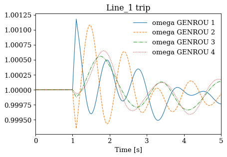
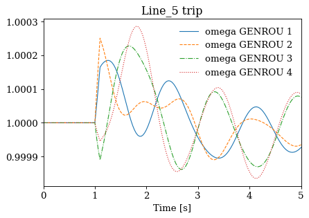
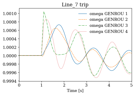
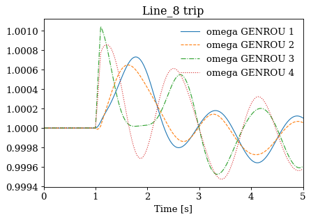
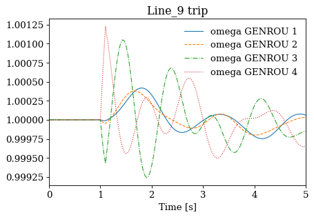
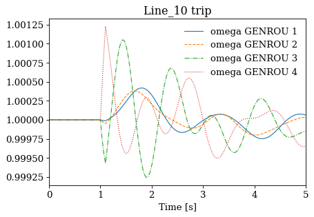
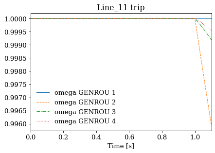
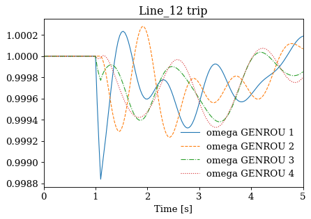
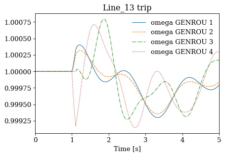
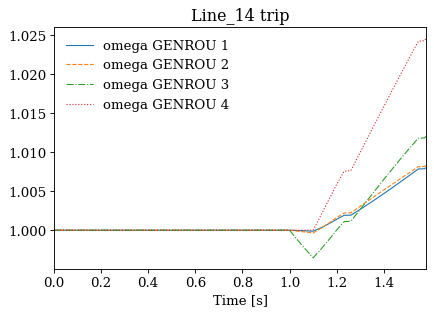
Not all cases will solve due to system instability. For the converged cases, one can export the data or plot results following Example 1.

for idx, ss in results.items():
    ss.TDS.plt.plot(ss.GENROU.omega, title=f'{idx} trip', latex=False, dpi=80)

!rm -rf batch_cases/