Load Frequency Control#
This examples shows (1) how to trip a generator, and (2) how to drive frequency back by load shedding.
import andes
import numpy as np

andes.config_logger(stream_level=20)
Tripping a Generator in the IEEE 14-Bus System#
# using the IEEE 14-bus model as an example.
# The example here contains a variety of models: generators, exciters, turbine governors, and PSS
# To speed up, one can remove unneeded ones, e.g., PSS

ieee14_raw = andes.get_case("ieee14/ieee14.raw")
ieee14_dyr = andes.get_case("ieee14/ieee14.dyr")
# use `andes.load` to load the test system
# Need to set `setup=False` to be able to add new Toggles that turns off generators.

ss = andes.load(ieee14_raw, addfile=ieee14_dyr, setup=False)
Working directory: "/home/hacui/repos/andes/examples"
> Loaded config from file "/home/hacui/.andes/andes.rc"
> Loaded generated Python code in "/home/hacui/.andes/pycode".
Parsing input file "/home/hacui/repos/andes/andes/cases/ieee14/ieee14.raw"...
  IEEE 14 BUS TEST CASE
  03/06/14 CONTO           100.0  1962 W
Input file parsed in 0.0119 seconds.
Parsing additional file "/home/hacui/repos/andes/andes/cases/ieee14/ieee14.dyr"...
Addfile parsed in 0.2965 seconds.
# Add a Toggle that disconnects `GENROU_2` at t=1 s

ss.add("Toggle", dict(model='SynGen', dev="GENROU_2", t=1.0))
'Toggle_3'
# Call setup manually

ss.setup()
IEEEST <IEEEST_1> added BusFreq <BusFreq_1> linked to bus <3.0>
ST2CUT <ST2CUT_2> added BusFreq <BusFreq_2> linked to bus <1.0>
ST2CUT <ST2CUT_3> added BusFreq <BusFreq_3> linked to bus <2.0>
System internal structure set up in 0.0750 seconds.
True
# double check that Toggles are set up correctly
# Check `u` of the Toggles - the first two line switches are disabled, and the generator trip is enabled

ss.Toggle.as_df()
| idx | u | name | model | dev | t | |
|---|---|---|---|---|---|---|
| uid | ||||||
| 0 | Toggle_1 | 1.0 | Toggle_1 | Line | Line_1 | 1.0 |
| 1 | Toggle_2 | 1.0 | Toggle_2 | Line | Line_1 | 1.1 |
| 2 | Toggle_3 | 1.0 | Toggle_3 | SynGen | GENROU_2 | 1.0 |
# disable existing line switches
# The IEEE 14-bus system contains predefined line switches. Disabling them to study generator trip only.

ss.Toggle.u.v[[0, 1]] = 0
# calculate power flow

# use constant power model for PQ (we will come back to this later)

ss.PQ.config.p2p = 1
ss.PQ.config.q2q = 1
ss.PQ.config.p2z = 0
ss.PQ.config.q2z = 0

# turn off under-voltage PQ-to-Z conversion
ss.PQ.pq2z = 0

ss.PFlow.run()
-> System connectivity check results:
  No islanded bus detected.
  System is interconnected.
  Each island has a slack bus correctly defined and enabled.

-> Power flow calculation
           Numba: Off
   Sparse solver: KLU
 Solution method: NR method
Power flow initialized in 0.0101 seconds.
0: |F(x)| = 0.5605182134
1: |F(x)| = 0.006202200332
2: |F(x)| = 5.819382824e-06
3: |F(x)| = 6.96508129e-12
Converged in 4 iterations in 0.0111 seconds.
Initialization for dynamics completed in 0.0575 seconds.
Initialization was successful.
Report saved to "ieee14_out.txt" in 0.0083 seconds.
True
# set the first simulation stop and run it

ss.TDS.config.tf = 20
ss.TDS.config.criteria = 0  # temporarily turn off stability criteria based on angle separation
ss.TDS.run()
-> Time Domain Simulation Summary:
Sparse Solver: KLU
Simulation time: 0.0-20 s.
Fixed step size: h=33.33 ms. Shrink if not converged.
<Toggle Toggle_3>: SynGen.GENROU_2 status changed to 0 at t=1.0 sec.
Simulation completed in 2.9748 seconds.
Outputs to "ieee14_out.lst" and "ieee14_out.npz".
Outputs written in 0.0421 seconds.
True
# Show the frequency response of online generators

# Refer to `plot` documentation by using `help(ss.TDS.plt.plot)` and `help(ss.TDS.plt.plot_data)`
ss.TDS.load_plotter()

ss.TDS.plt.plot(ss.GENROU.omega,
                a=(0, 2, 3, 4),
                ytimes=60,
               )
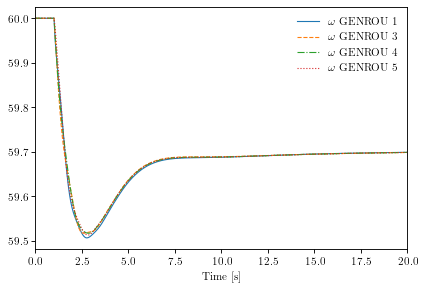
(<Figure size 480x320 with 1 Axes>, <AxesSubplot:xlabel='Time [s]'>)
Adjusting Load to Compensate for the Generation Loss#
Check the power of the lost generator by inspecting the power flow inputs:
ss.PV.as_df()
| idx | u | name | Sn | Vn | bus | busr | p0 | q0 | pmax | pmin | qmax | qmin | v0 | vmax | vmin | ra | xs | |
|---|---|---|---|---|---|---|---|---|---|---|---|---|---|---|---|---|---|---|
| uid | ||||||||||||||||||
| 0 | 2 | 0.0 | 2 | 100.0 | 69.0 | 2 | None | 0.40 | 0.15 | 0.5 | 0.1 | 0.15 | -0.40 | 1.03 | 1.4 | 0.6 | 0.0 | 0.13 |
| 1 | 3 | 0.0 | 3 | 100.0 | 69.0 | 3 | None | 0.40 | 0.15 | 0.5 | 0.1 | 0.15 | -0.10 | 1.01 | 1.4 | 0.6 | 0.0 | 0.13 |
| 2 | 4 | 0.0 | 4 | 100.0 | 138.0 | 6 | None | 0.30 | 0.10 | 0.5 | 0.1 | 0.10 | -0.06 | 1.03 | 1.4 | 0.6 | 0.0 | 0.12 |
| 3 | 5 | 0.0 | 5 | 100.0 | 69.0 | 8 | None | 0.35 | 0.10 | 0.5 | 0.1 | 0.10 | -0.06 | 1.03 | 1.4 | 0.6 | 0.0 | 0.12 |
The tripped GENROU_2 correspond to the first PV (GENROU_1 corresponds to Slack). Thus, the lost active power is 0.40 pu.
Let's compensate for that by shedding 0.4 pu of active power load at t=2.0 s.
By checking the equation documentation of PQ (using print(ss.PQ.doc()), we can tell that the imposed active power for time-domain simulation is from Ppf, because we used the constant power model with p2p = 1.
Algebraic Equations

Name |   Type   |                RHS of Equation "0 = g(x, y)"
-----+----------+-------------------------------------------------------------
 a   | ExtAlgeb | u * (dae_t <= 0) * (p0 * vcmp_zi + Rlb * vcmp_zl * v**2 +
     |          | Rub * vcmp_zu * v**2) + u * (dae_t > 0) * (p2p * Ppf + p2i *
     |          | Ipeq * v + p2z * Req * v**2)
 v   | ExtAlgeb | u * (dae_t <= 0) * (q0 * vcmp_zi + Xlb * vcmp_zl * v**2 +
     |          | Xub * vcmp_zu * v**2) + u * (dae_t > 0) * (q2q * Qpf + q2i *
     |          | Iqeq * v + q2z * Xeq * v**2)
Ppf may be different from p0 specified in the data file.
# active power from power flow solution - make a copy

Ppf = np.array(ss.PQ.Ppf.v)

Ppf
array([0.217, 0.5  , 0.478, 0.076, 0.15 , 0.295, 0.09 , 0.035, 0.061,
       0.135, 0.2  ])
Reload the system and add the generator trip.
ss = andes.load(ieee14_raw, addfile=ieee14_dyr, setup=False)

ss.add("Toggle", dict(model='SynGen', dev="GENROU_2", t=1.0))
ss.setup()
ss.Toggle.u.v[[0, 1]] = 0

ss.PQ.config.p2p = 1
ss.PQ.config.q2q = 1
ss.PQ.config.p2z = 0
ss.PQ.config.q2z = 0
ss.PQ.pq2z = 0

ss.PFlow.run()
Working directory: "/home/hacui/repos/andes/examples"
> Loaded config from file "/home/hacui/.andes/andes.rc"
> Reloaded generated Python code of module "pycode".
Parsing input file "/home/hacui/repos/andes/andes/cases/ieee14/ieee14.raw"...
  IEEE 14 BUS TEST CASE
  03/06/14 CONTO           100.0  1962 W
Input file parsed in 0.0047 seconds.
Parsing additional file "/home/hacui/repos/andes/andes/cases/ieee14/ieee14.dyr"...
Addfile parsed in 0.1101 seconds.
IEEEST <IEEEST_1> added BusFreq <BusFreq_1> linked to bus <3.0>
ST2CUT <ST2CUT_2> added BusFreq <BusFreq_2> linked to bus <1.0>
ST2CUT <ST2CUT_3> added BusFreq <BusFreq_3> linked to bus <2.0>
System internal structure set up in 0.0547 seconds.
-> System connectivity check results:
  No islanded bus detected.
  System is interconnected.
  Each island has a slack bus correctly defined and enabled.

-> Power flow calculation
           Numba: Off
   Sparse solver: KLU
 Solution method: NR method
Power flow initialized in 0.0040 seconds.
0: |F(x)| = 0.5605182134
1: |F(x)| = 0.006202200332
2: |F(x)| = 5.819382824e-06
3: |F(x)| = 6.96508129e-12
Converged in 4 iterations in 0.0065 seconds.
Initialization for dynamics completed in 0.0547 seconds.
Initialization was successful.
Report saved to "ieee14_out.txt" in 0.0028 seconds.
True
But let's run to 2 seconds.
ss.TDS.config.tf = 2.0
ss.TDS.config.criteria = 0  # temporarily turn off stability criteria based on angle separation

ss.TDS.run()
-> Time Domain Simulation Summary:
Sparse Solver: KLU
Simulation time: 0.0-2.0 s.
Fixed step size: h=33.33 ms. Shrink if not converged.
<Toggle Toggle_3>: SynGen.GENROU_2 status changed to 0 at t=1.0 sec.
Simulation completed in 0.2567 seconds.
Outputs to "ieee14_out.lst" and "ieee14_out.npz".
Outputs written in 0.0043 seconds.
True
# all `Ppf` before shedding

ss.PQ.Ppf.v
array([0.217, 0.5  , 0.478, 0.076, 0.15 , 0.295, 0.09 , 0.035, 0.061,
       0.135, 0.2  ])
And then apply the load shedding on buses 2, 3, 4, 5, 6, 9.
shed_buses = [2, 3, 4, 5, 6, 9]

# find the `idx` of the loads on these buses

pq_shed_idx = ss.PQ.find_idx(keys='bus', values=shed_buses)
pq_shed_idx
['PQ_1', 'PQ_2', 'PQ_3', 'PQ_4', 'PQ_5', 'PQ_6']
# get `Ppf` on these buses before shedding

pq_p = ss.PQ.get(src='Ppf', idx=pq_shed_idx, attr='v')
pq_p
array([0.217, 0.5 , 0.478, 0.076, 0.15 , 0.295])
pq_p_new = pq_p - 0.4 / len(shed_buses)

ss.PQ.set(src='Ppf', idx=pq_shed_idx, attr='v', value=pq_p_new)
True
# double check

ss.PQ.Ppf.v
array([0.15033333, 0.43333333, 0.41133333, 0.00933333, 0.08333333,
       0.22833333, 0.09      , 0.035     , 0.061     , 0.135     ,
       0.2       ])
ss.TDS.config.tf = 10

ss.TDS.run()

ss.TDS.plt.plot(ss.GENROU.omega,
                a=(0, 2, 3, 4),
                ytimes=60,
               )
Simulation completed in 1.2884 seconds.
Outputs to "ieee14_out.lst" and "ieee14_out.npz".
Outputs written in 0.0211 seconds.
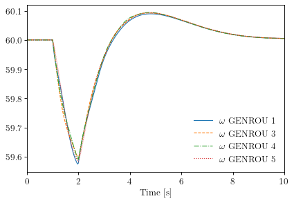
(<Figure size 480x320 with 1 Axes>, <AxesSubplot:xlabel='Time [s]'>)
!andes misc -C
"/home/hacui/repos/andes/examples/ieee14_out.txt" removed.
"/home/hacui/repos/andes/examples/ieee14_out.lst" removed.
"/home/hacui/repos/andes/examples/ieee14_out.npz" removed.
The result shows the generator speed (frequency) returns to 60 Hz after load shedding.