Examples#
We show two examples to demonstrate modeling from equations and modeling from control block diagrams.
The TGOV1 example shows code snippet for equation-based modeling and, as well as code for block-based modeling.
The IEEEST example walks through the source code and explains the complete setup, including optional parameters, input selection, and manual per-unit conversion.
TGOV1#
The TGOV1 turbine governor model is shown as a practical example using the library.
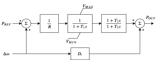
This model is composed of a lead-lag transfer function and a first-order lag transfer function with an anti-windup limiter, which are sufficiently complex for demonstration. The corresponding differential equations and algebraic equations are given below.
where LG and LL denote the lag block and the lead-lag block, \(\dot{x}_{LG}\) and \(\dot{x}_{LL}\) are the internal states, \(y_{LL}\) is the lead-lag output, \(\omega\) the generator speed, \(\omega_d\) the generator under-speed, \(P_d\) the droop output, \(\tau_{m0}\) the steady-state torque input, and \(P_{OUT}\) the turbine output that will be summed at the generator.
The code to describe the above model using equations is given below.
The complete code can be found in class TGOV1ModelAlt in
andes/models/governor.py.
def __init__(self, system, config):
  # 1. Declare parameters from case file inputs.
  self.R = NumParam(info='Turbine governor droop',
                    non_zero=True, ipower=True)
  # Other parameters are omitted.

  # 2. Declare external variables from generators.
  self.omega = ExtState(src='omega',
                 model='SynGen',
                 indexer=self.syn,
                 info='Generator speed')
  self.tm = ExtAlgeb(src='tm',
              model='SynGen',
              indexer=self.syn,
              e_str='u*(pout-tm0)',
              info='Generator torque input')

  # 3. Declare initial values from generators.
  self.tm0 = ExtService(src='tm',
               model='SynGen',
               indexer=self.syn,
               info='Initial torque input')

  # 4. Declare variables and equations.
  self.pref = Algeb(info='Reference power input',
                v_str='tm0*R',
                e_str='tm0*R-pref')
  self.wd = Algeb(info='Generator under speed',
              e_str='(1-omega)-wd')
  self.pd = Algeb(info='Droop output',
              v_str='tm0',
              e_str='(wd+pref)/R-pd')
  self.LG_x = State(info='State in the lag TF',
                v_str='pd',
                e_str='LG_lim_zi*(pd-LG_x)/T1')
  self.LG_lim = AntiWindup(u=self.LG_x,
                  lower=self.VMIN,
                  upper=self.VMAX)
  self.LL_x = State(info='State in the lead-lag TF',
                v_str='LG_x',
                e_str='(LG_x-LL_x)/T3')
  self.LL_y = Algeb(info='Lead-lag Output',
                v_str='LG_x',
                e_str='T2/T3*(LG_x-LL_x)+LL_x-LL_y')
  self.pout = Algeb(info='Turbine output power',
                v_str='tm0',
                e_str='(LL_y+Dt*wd)-pout')
Another implementation of TGOV1 makes extensive use of the modeling blocks. The resulting code is more readable as follows.
def __init__(self, system, config):
    TGBase.__init__(self, system, config)

    self.gain = ConstService(v_str='u/R')

    self.pref = Algeb(info='Reference power input',
                      tex_name='P_{ref}',
                      v_str='tm0 * R',
                      e_str='tm0 * R - pref',
                      )

    self.wd = Algeb(info='Generator under speed',
                    unit='p.u.',
                    tex_name=r'\omega_{dev}',
                    v_str='0',
                    e_str='(wref - omega) - wd',
                    )
    self.pd = Algeb(info='Pref plus under speed times gain',
                    unit='p.u.',
                    tex_name="P_d",
                    v_str='u * tm0',
                    e_str='u*(wd + pref + paux) * gain - pd')

    self.LAG = LagAntiWindup(u=self.pd,
                             K=1,
                             T=self.T1,
                             lower=self.VMIN,
                             upper=self.VMAX,
                             )

    self.LL = LeadLag(u=self.LAG_y,
                      T1=self.T2,
                      T2=self.T3,
                      )

    self.pout.e_str = '(LL_y + Dt * wd) - pout'
The complete code can be found in class TGOV1Model in andes/models/governor.py.
IEEEST#
In this example, we will explain step-by-step how IEEEST is programmed.
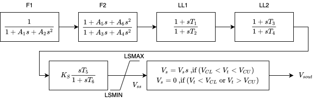
The block diagram of IEEEST is given as follows.
We recommend you to open up the source code in andes/models/pss.py and
then continue reading.
First of all, modeling components are imported at the beginning.
Next, PSSBaseData is defined to hold parameters shared by all PSSs.
PSSBaseData inherits from ModelData and calls the base constructor.
There is only one field avr defined for the linked exciter idx.
Then, IEEESTData defines the input parameters for IEEEST.
Use IdxParam for fields that store idx-es of devices that IEEEST devices link to.
Use NumParam for numerical parameters.
PSSBase#
PSSBase is defined for the common (external) parameters, services and variables
shared by all PSSs.
The class and constructor signatures are
class PSSBase(Model):
    def __init__(self, system, config):
        super().__init__(system, config)
PSSBase inherits from Model and calls the base constructor.
Note that the call to Model's constructor takes two positional arguments, system
and config of types System and ModelConfig.
Next, the group is specified, and the model flags are set.
Note
It is important to set the TDS flag to register the model. If not set, data for the model will be successfully loaded, but the variables in the model will not receive any address, and the model equations will be skipped.
There is a similar flag self.flags.pflow for models to participate in
power flow calculations. Most dynamic models, however, are initialized after
power flow.
self.group = 'PSS'
self.flags.tds = True
Next, Replace is used to replace input parameters that satisfy a lambda function
with new values.
self.VCUr = Replace(self.VCU, lambda x: np.equal(x, 0.0), 999)
self.VCLr = Replace(self.VCL, lambda x: np.equal(x, 0.0), -999)
The value replacement happens when VCUr and VCLr is first accessed.
Replace is executed in the model initialization phase (at the end of
services update).
Next, the indices of connected generators, buses, and bus frequency measurements are retrieved. Synchronous generator idx is retrieved with
self.syn = ExtParam(model='Exciter', src='syn', indexer=self.avr, export=False,
                    info='Retrieved generator idx', vtype=str)
Using the retrieved self.syn, it retrieves the buses to which
the generators are connected.
self.bus = ExtParam(model='SynGen', src='bus', indexer=self.syn, export=False,
                    info='Retrieved bus idx', vtype=str, default=None,
                    )
PSS models support an optional remote bus specified through parameter busr.
When busr is None, the generator-connected bus should be used.
The following code uses DataSelect to select busr if available but falls
back to bus otherwise.
self.buss = DataSelect(self.busr, self.bus, info='selected bus (bus or busr)')
Each PSS links to a bus frequency measurement device.
If the input data does not specify one or the specified one does not exist,
DeviceFinder can find the correct measurement device for the bus
where frequency measurements should be taken.
self.busfreq = DeviceFinder(self.busf, link=self.buss, idx_name='bus')
where busf is the optional frequency measurement device idx, buss is the bus idx
for which measurement device needs to be found or created.
Next, external parameters, variables and services are retrieved.
Note that the PSS output vsout is pre-allocated but the equation string
is left to specific models.
IEEESTModel#
IEEESTModel inherits from PSSBase and adds specific model components.
After calling PSSBase's constructor, IEEESTModel adds config entries
to allow specifying the model for frequency measurement, because
there may be multiple frequency measurement models in the future.
self.config.add(OrderedDict([('freq_model', 'BusFreq')]))
self.config.add_extra('_help', {'freq_model': 'default freq. measurement model'})
self.config.add_extra('_alt', {'freq_model': ('BusFreq',)})
We set the chosen measurement model to busf so that DeviceFinder knows which
model to use if it needs to create new devices.
self.busf.model = self.config.freq_model
Next, because bus voltage is an algebraic variable, we use Derivative to calculate
the finite difference to approximate its derivative.
self.dv = Derivative(self.v, tex_name='dV/dt', info='Finite difference of bus voltage')
Then, we retrieve the coefficient to convert power from machine base to system base
using ConstService, given by Sb / Sn.
This is needed for input mode 3, electric power in machine base.
self.SnSb = ExtService(model='SynGen', src='M', indexer=self.syn, attr='pu_coeff',
                       info='Machine base to sys base factor for power',
                       tex_name='(Sb/Sn)')
Note that the ExtService access the pu_coeff field of the M variables of
synchronous generators.
Since M is a machine-base power quantity, M.pu_coeff stores the multiplication coefficient
to convert each of them from machine bases to the system base, which is Sb / Sn.
The input mode is parsed into boolean flags using Switcher:
self.SW = Switcher(u=self.MODE,
                   options=[0, 1, 2, 3, 4, 5, 6],
                   )
where the input u is the MODE parameter, and options is a list of accepted
values.
Switcher boolean arrays s0, s1, ..., sN, where N = len(options) - 1.
We added 0 to options for padding so that SW_s1 corresponds to MODE 1.
It improves the readability of the code as we will see next.
The input signal sig is an algebraic variable given by
self.sig = Algeb(tex_name='S_{ig}',
                 info='Input signal',
                 )

self.sig.v_str = 'SW_s1*(omega-1) + SW_s2*0 + SW_s3*(tm0/SnSb) + ' \
                 'SW_s4*(tm-tm0) + SW_s5*v + SW_s6*0'

self.sig.e_str = 'SW_s1*(omega-1) + SW_s2*(f-1) + SW_s3*(te/SnSb) + ' \
                 'SW_s4*(tm-tm0) + SW_s5*v + SW_s6*dv_v - sig'
The v_str and e_str are separated from the constructor to improve readability.
They construct piece-wise functions to select the correct initial values and equations
based on mode.
For any variables in v_str, they must be defined before sig so that
they will be initialized ahead of sig.
Clearly, omega, tm, and v are defined in PSSBase and thus
come before sig.
The following comes the most effective part: modeling using transfer function blocks.
We utilized several blocks to describe the model from the diagram.
Note that the output of a block is always the block name followed by _y.
For example, the input of F2 is the output of F1, given by F1_y.
self.F1 = Lag2ndOrd(u=self.sig, K=1, T1=self.A1, T2=self.A2)

self.F2 = LeadLag2ndOrd(u=self.F1_y, T1=self.A3, T2=self.A4,
                        T3=self.A5, T4=self.A6, zero_out=True)

self.LL1 = LeadLag(u=self.F2_y, T1=self.T1, T2=self.T2, zero_out=True)

self.LL2 = LeadLag(u=self.LL1_y, T1=self.T3, T2=self.T4, zero_out=True)

self.Vks = Gain(u=self.LL2_y, K=self.KS)

self.WO = WashoutOrLag(u=self.Vks_y, T=self.T6, K=self.T5, name='WO',
                       zero_out=True)  # WO_y == Vss

self.VLIM = Limiter(u=self.WO_y, lower=self.LSMIN, upper=self.LSMAX,
                    info='Vss limiter')

self.Vss = Algeb(tex_name='V_{ss}', info='Voltage output before output limiter',
                 e_str='VLIM_zi * WO_y + VLIM_zu * LSMAX + VLIM_zl * LSMIN - Vss')

self.OLIM = Limiter(u=self.v, lower=self.VCLr, upper=self.VCUr,
                    info='output limiter')

self.vsout.e_str = 'OLIM_zi * Vss - vsout'
In the end, the output equation is assigned to vsout.e_str.
It completes the equations of the IEEEST model.
Finalize#
Assemble IEEESTData and IEEESTModel into IEEEST:
class IEEEST(IEEESTData, IEEESTModel):
    def __init__(self, system, config):
        IEEESTData.__init__(self)
        IEEESTModel.__init__(self, system, config)
Locate and edit the file andes/models/__init__.py. The variable
file_classes is a list of tuples that stores the source file and class names
in strings. In each tuple, the first element is the .py file name in the
models folder, and the second element is a list of class names to be
imported from that file.
Find the line with pss, then add IEEEST to the corresponding list of
model names. The line will look like
file_classes = list([
    ...
    ('pss', ['IEEEST', 'ST2CUT']),
    ...
])
Note in the above that the string 'IEEEST' is used. The line above is valid
as long as from andes.models.pss import IEEEST is valid. If the source file
name does not exist in any line of file_classes, one may add it after all
prerequisite models. For example, the pss line should be added after
exciters (and generators, of course).
Finally, locate andes/models/group.py, check if the class PSS exist. It
needs to match the group name of IEEEST. If not, create one by inheriting from
GroupBase:
class PSS(GroupBase):
    """Power system stabilizer group."""

    def __init__(self):
        super().__init__()
        self.common_vars.extend(('vsout',))
where we added vsout to the common_vars list. All models in the PSS
group must have a variable named vsout, which is defined in PSSBase.
This completes the IEEEST model. When developing new models, use andes
prepare to generate numerical code and start debugging.