Forced Oscillation Source Localization

Forced oscillations in power systems arise when a periodic disturbance, such as a malfunctioning governor valve, injects energy at a fixed frequency. Unlike natural oscillations, forced oscillations persist as long as the source remains active, and resonance can amplify the response at generators far from the source. Locating the source from measurements alone is therefore a non-trivial problem.

This notebook demonstrates two PMU-based methods on a 179-bus WECC system with 29 generators:

1. Energy flow analysis: the dissipating energy flow (DEF) method computes \(E_i = \int \Delta P_{e,i} \cdot \Delta\omega_i\, dt\) at each generator; the source is the only generator with a positive value [1, 2].

2. Phase difference analysis: the \(P_e\)–\(\omega\) phase difference at the source is a clear outlier relative to all other generators [2].

Both methods use only bus frequency and electrical power, quantities directly observable from phasor measurement units.

References

[1] S. Maslennikov, B. Wang, and E. Litvinov, "Dissipating energy flow method for locating the source of sustained oscillations," Int. J. Elect. Power Energy Syst., vol. 88, pp. 55–62, Jun. 2017.

[2] L. Chen, Y. Min, and W. Hu, "An energy-based method for location of power system oscillation source," IEEE Trans. Power Syst., vol. 28, no. 2, pp. 828–836, May 2013.

Show code cell source

Hide code cell source

%matplotlib inline

import numpy as np
from scipy import signal
from pathlib import Path
from matplotlib import pyplot as plt

import andes

andes.config_logger(stream_level=30)

System Setup

The WECC 179-bus system is loaded from PSS/E format files originally provided by Kai Sun's Oscillation Test Cases Library. The model contains 29 GENCLS generators with uniform damping (\(D = 4\)). A TGOV1 governor is added to each generator to provide realistic mechanical power dynamics, and BusFreq devices are installed at all generator buses.

case_dir = Path("cases/wecc179")
ss = andes.load(str(case_dir / "wecc179.raw"),
                addfile=str(case_dir / "wecc179.dyr"), setup=False)

gen_buses = list(ss.GENCLS.bus.v)
gen_idxs = list(ss.GENCLS.idx.v)
n_gen = len(gen_idxs)

for idx in gen_idxs:
    ss.add("TGOV1", syn=idx, R=0.05, T1=0.5, T2=1.0,
           T3=2.0, Dt=0.0, VMAX=99, VMIN=0)

for bus in gen_buses:
    ss.add("BusFreq", bus=bus)

ss.setup()
ss.PFlow.run()

True

Periodic Disturbance Injection

A square-wave disturbance at 0.37 Hz is applied to the auxiliary power input of the generator at bus 77. This frequency coincides with a natural electromechanical mode of the system, producing resonance. Due to resonance, generators far from the source may oscillate with comparable or even larger amplitude, making amplitude-based source identification unreliable.

source_bus = 77
source_idx = dict(zip(gen_buses, gen_idxs))[source_bus]

f_osc = 0.37
half_period = 1.0 / (2 * f_osc)
amplitude = 0.03
t_start, t_end = 2.0, 42.0

ss.config.warn_abnormal = 0
ss.TDS.config.tf = t_start
ss.TDS.config.no_tqdm = 1
ss.TDS.run()

t = t_start
positive = True
while t + half_period <= t_end:
    ss.SynGen.set_paux(ss, source_idx, amplitude if positive else -amplitude)
    t += half_period
    ss.TDS.config.tf = t
    ss.TDS.run()
    positive = not positive

ss.SynGen.set_paux(ss, source_idx, 0.0)
ss.TDS.config.tf = t_end + 5.0
ss.TDS.run()

True

Observing the Forced Oscillation

Show code cell source

Hide code cell source

ts_bf = ss.TDS.get_timeseries(ss.BusFreq.f)
bf_buses = list(ss.BusFreq.bus.v)

fig, axes = plt.subplots(2, 1, figsize=(10, 5), sharex=True)

for i in range(len(bf_buses)):
    axes[0].plot(ts_bf.index, ts_bf.iloc[:, i], alpha=0.4, linewidth=0.5)
axes[0].set_ylabel("Frequency [pu]")
axes[0].set_title("Bus frequency at all 29 generator buses")

source_col = bf_buses.index(source_bus)
remote_col = bf_buses.index(35)

axes[1].plot(ts_bf.index, ts_bf.iloc[:, source_col],
             label=f"Source (bus {source_bus})")
axes[1].plot(ts_bf.index, ts_bf.iloc[:, remote_col],
             label="Bus 35 (largest non-source response)", alpha=0.7)
axes[1].set_ylabel("Frequency [pu]")
axes[1].set_xlabel("Time [s]")
axes[1].legend()

plt.tight_layout()

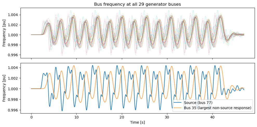
All 29 generator buses exhibit oscillations at the forcing frequency. The amplitude at bus 35 exceeds that at the source (bus 77), illustrating the resonance amplification effect. This behavior renders simple amplitude comparison unreliable for source identification and motivates the energy-based and phase-based methods developed below.

Spectral Analysis

Show code cell source

Hide code cell source

time = ts_bf.index.values
mask = (time >= 5.0) & (time <= t_end)
t_ss = time[mask]
dt = np.median(np.diff(t_ss))
N = len(t_ss)

bf_ss = ts_bf.loc[mask].values
freqs = np.fft.rfftfreq(N, d=dt)

fig, ax = plt.subplots(figsize=(6, 4))
for i, bus in enumerate(bf_buses):
    spectrum = np.abs(np.fft.rfft(bf_ss[:, i] - bf_ss[:, i].mean())) * 2 / N
    is_src = bus == source_bus
    ax.plot(freqs, spectrum,
            alpha=0.9 if is_src else 0.3,
            linewidth=1.5 if is_src else 0.5,
            color="#d62728" if is_src else "#1f77b4",
            label=f"Bus {bus} (source)" if is_src else None)

ax.set_xlim(0, 2.0)
ax.set_xlabel("Frequency [Hz]")
ax.set_ylabel("Amplitude [pu]")
ax.set_title("Frequency spectrum at all generator buses")
ax.axvline(f_osc, color="gray", linestyle="--", alpha=0.5,
           label=f"Forcing: {f_osc} Hz")
ax.legend()
plt.tight_layout()

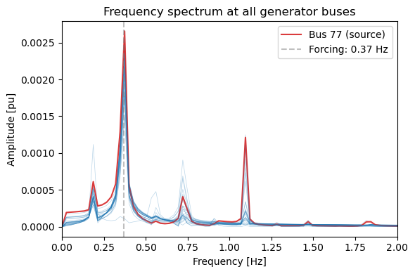
A sharp spectral peak at 0.37 Hz is present at all generator buses, confirming the forced oscillation frequency. The peak amplitudes are comparable across buses, reinforcing the observation that amplitude alone cannot identify the source.

Energy-Based Source Localization

The oscillation energy flow at each generator is computed as

\[E_i = \int \Delta P_{e,i}(t) \cdot \Delta\omega_i(t)\, dt\]

where \(\Delta P_{e,i}\) and \(\Delta\omega_i\) are bandpass-filtered oscillatory components of electrical power and rotor speed. A generator that injects oscillation energy into the network (the source) yields a positive value, while generators that absorb energy yield negative values.

ts_Pe = ss.TDS.get_timeseries(ss.GENCLS.Pe)
ts_omega = ss.TDS.get_timeseries(ss.GENCLS.omega)

Pe_ss = ts_Pe.loc[mask].values
omega_ss = ts_omega.loc[mask].values

fs = 1.0 / dt
sos = signal.butter(4, [max(f_osc - 0.1, 0.05), f_osc + 0.1],
                    btype="bandpass", fs=fs, output="sos")

energy = np.zeros(n_gen)
for j in range(n_gen):
    pe_filt = signal.sosfiltfilt(sos, Pe_ss[:, j])
    om_filt = signal.sosfiltfilt(sos, omega_ss[:, j] - 1.0)
    energy[j] = np.trapezoid(pe_filt * om_filt, t_ss)

Show code cell source

Hide code cell source

bus_labels = [str(b) for b in gen_buses]
colors = ["red" if b == source_bus else "steelblue" for b in gen_buses]

fig, ax = plt.subplots(figsize=(12, 4))
ax.bar(bus_labels, energy, color=colors)
ax.set_xlabel("Generator bus")
ax.set_ylabel(r"$E_i = \int \Delta P_e \cdot \Delta\omega\, dt$")
ax.set_title("Oscillation energy flow at each generator")
ax.axhline(0, color="black", linewidth=0.5)
plt.xticks(rotation=45, fontsize=7)
plt.tight_layout()

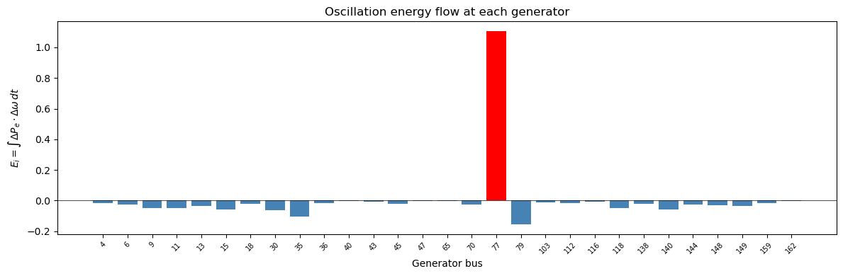
The source generator at bus 77 (red) is the only generator with a positive energy flow, indicating that it injects oscillation energy into the network. All remaining 28 generators have negative values, meaning they absorb energy from the oscillation. The margin is decisive: the source energy exceeds +1.1, while the next-closest generator is near zero.

Phase-Based Confirmation

The phase difference between electrical power and rotor speed oscillations at the forcing frequency provides an independent confirmation of the source location. At the source, the \(P_e\)–\(\omega\) phase difference deviates substantially from the cluster formed by all other generators.

Show code cell source

Hide code cell source

f_idx = np.argmin(np.abs(freqs - f_osc))

phase_diff = np.zeros(n_gen)
for j in range(n_gen):
    fft_pe = np.fft.rfft(Pe_ss[:, j] - Pe_ss[:, j].mean())
    fft_om = np.fft.rfft(omega_ss[:, j] - omega_ss[:, j].mean())
    diff = np.angle(fft_pe[f_idx]) - np.angle(fft_om[f_idx])
    phase_diff[j] = np.degrees(np.arctan2(np.sin(diff), np.cos(diff)))

Show code cell source

Hide code cell source

fig, ax = plt.subplots(figsize=(12, 4))
ax.bar(bus_labels, phase_diff, color=colors)
ax.set_xlabel("Generator bus")
ax.set_ylabel("Phase($P_e$) - Phase($\\omega$) [degrees]")
ax.set_title(f"$P_e$ - $\\omega$ phase difference at {f_osc} Hz")
plt.xticks(rotation=45, fontsize=7)
plt.tight_layout()

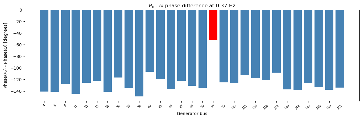
The source generator at bus 77 exhibits a \(P_e\)–\(\omega\) phase difference of approximately \(-52°\), while all other generators cluster between \(-107°\) and \(-149°\). This distinct outlier position provides unambiguous identification of the source, independent of and consistent with the energy flow result.

Extend This Example

• Change the forcing frequency away from resonance and observe how the energy flow margins change.

• Relocate the source to a different generator and verify that both methods correctly identify the new location.

• Add measurement noise to test robustness under realistic PMU conditions.

• Apply to field PMU data from actual forced oscillation events documented in Kai Sun's Oscillation Test Cases Library.