Physics-Informed Surrogate from Symbolic Equations#
Surrogate models that respect the governing physics can accelerate repeated simulation studies such as contingency screening and sensitivity analysis. A key challenge is encoding the differential- algebraic equations (DAEs) of the power system into a differentiable form suitable for neural network training.
ANDES stores every model equation as a symbolic string. Calling
model.prepare() parses these strings into SymPy expressions, which
can then be manipulated algebraically and converted to PyTorch
functions via sp.lambdify. This notebook demonstrates the complete
pipeline:
Extract the GENCLS differential and algebraic equations from ANDES.
Eliminate the 12 internal algebraic variables with
sp.solve.Convert the reduced ODE residual to a differentiable PyTorch function with
sp.lambdify.Train a parameterized Physics-Informed Neural Network (PINN) using the auto-derived residual as the physics loss.
No physics is hand-coded in PyTorch. The entire residual is derived programmatically from the ANDES model definition.
Device: cuda
Step 1 — Extract Symbolic Equations#
A single-machine infinite-bus (SMIB) system is constructed using the
ANDES v2 API. After power flow and TDS initialization, calling
gen.prepare() parses the e_str attributes of every GENCLS variable
into SymPy expressions stored in syms.f_list (differential) and
syms.g_list (algebraic).
ss = andes.System(default_config=True)
ss.undill()

ss.add("Bus", idx=1, name="Gen Bus", Vn=20.0, v0=1.0)
ss.add("Bus", idx=2, name="Inf Bus", Vn=20.0, v0=1.0)
ss.add("Line", idx=1, bus1=1, bus2=2, Vn1=20.0, Vn2=20.0,
       r=0.0, x=0.3, b=0.0)
ss.add("PV", idx=1, bus=1, Vn=20.0, p0=0.5, q0=0.0, v0=1.0)
ss.add("Slack", idx=2, bus=2, Vn=20.0, v0=1.0)
ss.add("GENCLS", idx=1, bus=1, gen=1, Sn=100, Vn=20.0,
       M=6.0, D=20.0, xd1=0.3, ra=0.0)

ss.setup()
ss.PFlow.run()
ss.TDS.init()

gen = ss.GENCLS
gen.prepare()

state_names = list(gen.cache.states_and_ext.keys())
algeb_names = list(gen.cache.algebs_and_ext.keys())

print("Differential equations (f_list)")
for i, name in enumerate(state_names):
    var = gen.cache.states_and_ext[name]
    tc = f" / {var.t_const.name}" if getattr(var, "t_const", None) else ""
    print(f"  d({name})/dt{tc} = {gen.syms.f_list[i]}")

print(f"\nAlgebraic equations ({len(algeb_names)} total, first 4 shown)")
for i in range(min(4, len(algeb_names))):
    print(f"  0 = {gen.syms.g_list[i]}")
Differential equations (f_list)
  d(delta)/dt = 2*pi*fn*ue*(omega - 1)
  d(omega)/dt / M = ue*(-D*(omega - 1) - te + tm)

Algebraic equations (14 total, first 4 shown)
  0 = Id*xq + psid - vf
  0 = Iq*xq + psiq
  0 = -ue*v*sin(a - delta) - vd
  0 = ue*v*cos(a - delta) - vq
Step 2 — Eliminate Algebraic Variables#
The GENCLS model has 12 internal algebraic variables (\(I_d\), \(I_q\),
\(v_d\), \(v_q\), \(t_e\), etc.) that couple the differential equations to
the network. These are eliminated automatically with sp.solve,
leaving an ODE in the state variables (\(\delta\), \(\omega\)) and the
external bus quantities (\(v\), \(a\)) that serve as parameters.
syms_d = gen.syms.inputs_dict

# Collect internal algebraic equations and variables
int_algeb = [n for n, v in gen.cache.algebs_and_ext.items()
             if not hasattr(v, "model")]
g_eqs = [gen.syms.g_list[i] for i, n in enumerate(algeb_names)
         if n in int_algeb]
g_vars = [syms_d[n] for n in int_algeb]

sol = sp.solve(g_eqs, g_vars, dict=True)[0]

# Substitute into both differential equations
f_delta_reduced = sp.simplify(gen.syms.f_list[0].subs(sol))
f_omega_reduced = sp.simplify(gen.syms.f_list[1].subs(sol))

print(f"Eliminated {len(sol)} algebraic variables")
print(f"\n  d(delta)/dt     = {f_delta_reduced}")
print(f"  M * d(omega)/dt = {f_omega_reduced}")
print(f"\nAuto-derived te = {sp.simplify(sol[syms_d['te']])}")
Eliminated 12 algebraic variables

  d(delta)/dt     = 2*pi*fn*ue*(omega - 1)
  M * d(omega)/dt = ue*(ue**4*vf0*(ra*ue*v*cos(a - delta) - ra*vf0 + v*xq*sin(a - delta)) - (D*(omega - 1) - tm0)*(ra**2*ue**2 + xq**2))/(ra**2*ue**2 + xq**2)

Auto-derived te = ue**4*vf0*(-ra*ue*v*cos(a - delta) + ra*vf0 - v*xq*sin(a - delta))/(ra**2*ue**2 + xq**2)
Step 3 — Convert to Differentiable PyTorch Functions#
The two reduced first-order ODEs from Step 2 are converted directly
to PyTorch-compatible functions via sp.lambdify. Machine constants
(\(M\), \(D\), \(x'_d\)) are fixed at their numerical values, while the
per-equilibrium coefficients (\(v_{f0}\), \(v\), \(a\), \(\tau_{m0}\)) are
kept symbolic so that the residuals can be evaluated across operating
points.
Each lambdify call produces a fully differentiable function that
supports torch.autograd. No manual algebraic manipulation is
performed; the ODEs are passed through as ANDES produced them.
# Fix machine constants, keep per-equilibrium params symbolic
const_subs = {
    syms_d["M"]: float(gen.M.v[0]),
    syms_d["D"]: float(gen.D.v[0]),
    syms_d["fn"]: float(ss.config.freq),
    syms_d["ue"]: 1.0,
    syms_d["ra"]: 0.0,
    syms_d["xq"]: float(gen.xd1.v[0]),
}

f_delta_num = sp.simplify(f_delta_reduced.subs(const_subs))
f_omega_num = sp.simplify(f_omega_reduced.subs(const_subs))
M_val = float(gen.M.v[0])

print(f"d(delta)/dt = {f_delta_num}")
print(f"d(omega)/dt = ({f_omega_num}) / {M_val}")
d(delta)/dt = 120.0*pi*(omega - 1)
d(omega)/dt = (-20.0*omega + 1.0*tm0 + 3.33333333333333*v*vf0*sin(a - delta) + 20.0) / 6.0
delta_s = syms_d["delta"]
omega_s = syms_d["omega"]
vf0_s = syms_d["vf0"]
v_s = syms_d["v"]
a_s = syms_d["a"]
tm0_s = syms_d["tm0"]

args = [delta_s, omega_s, vf0_s, v_s, a_s, tm0_s]

f_delta_torch = sp.lambdify(args, f_delta_num, modules=[TORCH_MODULES, "numpy"])
f_omega_torch = sp.lambdify(args, f_omega_num, modules=[TORCH_MODULES, "numpy"])

# Quick autograd check
d_test = torch.tensor(0.3, dtype=DTYPE, requires_grad=True)
o_test = torch.tensor(1.0, dtype=DTYPE, requires_grad=True)
vf0_t = torch.tensor(float(gen.vf0.v[0]), dtype=DTYPE)
v_t = torch.tensor(float(ss.Bus.v.v[0]), dtype=DTYPE)
a_t = torch.tensor(float(ss.Bus.a.v[0]), dtype=DTYPE)
tm0_t = torch.tensor(float(gen.tm0.v[0]), dtype=DTYPE)

ro = f_omega_torch(d_test, o_test, vf0_t, v_t, a_t, tm0_t)
ro.backward()
print(f"sp.lambdify -> PyTorch OK, autograd: d(f_omega)/d(delta) = {d_test.grad.item():.4f}")
sp.lambdify -> PyTorch OK, autograd: d(f_omega)/d(delta) = -3.3699
Step 4 — Train a Parameterized PINN#
The PINN learns the solution surface \((\delta, \omega)(P_m, t)\) across a range of mechanical power setpoints. ANDES TDS generates the ground-truth trajectories (with a 3-cycle fault at \(t = 0.1\) s); the auto-derived residuals from Step 3 provide the physics loss.
For each \(P_m\), a separate power flow is solved to obtain the per-equilibrium coefficients (\(v_{f0}\), \(v\), \(a\), \(\tau_{m0}\)). These are interpolated to each collocation point so that the physics loss reflects the correct equilibrium at every \(P_m\).
Element |
Value |
|---|---|
Network |
3-layer MLP, 256 units, tanh, 2 outputs |
Input / Output |
\((P_m,\, t) \to (\delta,\, \omega)\) |
Supervised points |
8 000 (20 \(P_m\) values \(\times\) 400 time steps) |
Collocation points |
8 000 (random, excluding fault window) |
Physics weight |
0.01 |
Optimizer |
Adam (5 000 epochs, cosine LR) + L-BFGS refinement |
Pm_sweep = np.linspace(0.1, 1.2, 20)
tf = 2.0
n_t = 400

print(f"Generating ground truth: {len(Pm_sweep)} Pm values, "
      f"tf={tf} s, 3-cycle fault at t=0.1 s")
t0 = time.time()

runs, valid_Pm = [], []
coeffs = {"vf0": [], "v": [], "a": [], "tm0": []}

for Pm in Pm_sweep:
    ret = build_smib(Pm, tf=tf)
    if ret is None:
        continue
    runs.append((ret["t"], ret["delta"], ret["omega"]))
    valid_Pm.append(Pm)
    for k in coeffs:
        coeffs[k].append(ret["coeff"][k])

t_vec = np.linspace(0.0, tf, n_t)
usol_delta = np.array([np.interp(t_vec, ti, di) for ti, di, _ in runs])
usol_omega = np.array([np.interp(t_vec, ti, oi) for ti, _, oi in runs])
Pm_vec = np.array(valid_Pm)
for k in coeffs:
    coeffs[k] = np.array(coeffs[k])

print(f"  {usol_delta.shape[0]} operating points x {usol_delta.shape[1]} "
      f"time steps, {time.time()-t0:.1f} s")
Generating ground truth: 20 Pm values, tf=2.0 s, 3-cycle fault at t=0.1 s
  20 operating points x 400 time steps, 3.3 s
Supervised: 8000 pts, Collocation: 8000 pts
def compute_physics_loss(model, X_f, coll_coeffs, M_val):
    """Physics loss enforcing both first-order ODEs."""
    X = X_f.clone().requires_grad_(True)
    out = model(X)                    # (N, 2): [delta, omega]
    delta_pred = out[:, 0:1]
    omega_pred = out[:, 1:2]

    # d(delta)/dt and d(omega)/dt via autograd
    ones = torch.ones_like(delta_pred)
    g_delta = torch.autograd.grad(delta_pred, X, ones, create_graph=True)[0]
    ddelta_dt = g_delta[:, 1:2]

    g_omega = torch.autograd.grad(omega_pred, X, ones, create_graph=True)[0]
    domega_dt = g_omega[:, 1:2]

    # RHS from auto-derived ANDES equations
    rhs_delta = f_delta_torch(
        delta_pred, omega_pred,
        coll_coeffs["vf0"], coll_coeffs["v"],
        coll_coeffs["a"], coll_coeffs["tm0"],
    )
    rhs_omega = f_omega_torch(
        delta_pred, omega_pred,
        coll_coeffs["vf0"], coll_coeffs["v"],
        coll_coeffs["a"], coll_coeffs["tm0"],
    ) / M_val

    res_delta = ddelta_dt - rhs_delta
    res_omega = domega_dt - rhs_omega

    return torch.mean(res_delta ** 2) + torch.mean(res_omega ** 2)


PHYS_WEIGHT = 0.01
ADAM_EPOCHS = 5000
hist = {"total": [], "data": [], "phys": []}
t0 = time.time()

# ── Adam phase ──
opt = torch.optim.Adam(model.parameters(), lr=1e-3)
sched = torch.optim.lr_scheduler.CosineAnnealingLR(
    opt, T_max=ADAM_EPOCHS, eta_min=1e-5)

for ep in range(1, ADAM_EPOCHS + 1):
    opt.zero_grad()
    ld = torch.mean((model(X_u) - y_u) ** 2)
    lp = compute_physics_loss(model, X_f, coll_coeffs, M_val)
    loss = ld + PHYS_WEIGHT * lp
    loss.backward()
    opt.step()
    sched.step()
    hist["total"].append(loss.item())
    hist["data"].append(ld.item())
    hist["phys"].append(lp.item())

print(f"Adam {ADAM_EPOCHS} epochs:  "
      f"data={ld.item():.2e}  phys={lp.item():.2e}")

# ── L-BFGS refinement ──
lbfgs = torch.optim.LBFGS(
    model.parameters(), max_iter=1000,
    max_eval=1250, tolerance_grad=1e-9,
    tolerance_change=1e-11, history_size=100,
    line_search_fn="strong_wolfe")

lbfgs_it = [0]

def closure():
    lbfgs.zero_grad()
    ld = torch.mean((model(X_u) - y_u) ** 2)
    lp = compute_physics_loss(model, X_f, coll_coeffs, M_val)
    loss = ld + PHYS_WEIGHT * lp
    loss.backward()
    lbfgs_it[0] += 1
    hist["total"].append(loss.item())
    hist["data"].append(ld.item())
    hist["phys"].append(lp.item())
    return loss

lbfgs.step(closure)

ld_f = torch.mean((model(X_u) - y_u) ** 2)
lp_f = compute_physics_loss(model, X_f, coll_coeffs, M_val)
print(f"L-BFGS {lbfgs_it[0]} iters: "
      f"data={ld_f.item():.2e}  phys={lp_f.item():.2e}")
print(f"Total training time: {time.time()-t0:.1f} s")
Adam 5000 epochs:  data=1.32e-05  phys=9.04e-04
L-BFGS 1030 iters: data=4.94e-07  phys=6.48e-04
Total training time: 260.9 s
Results#
The trained PINN is evaluated against the ANDES TDS ground truth across the full \((P_m, t)\) domain.
delta:  MAE = 0.037 deg,  max error = 0.456 deg
omega:  MAE = 0.000063 pu,   max error = 0.001948 pu
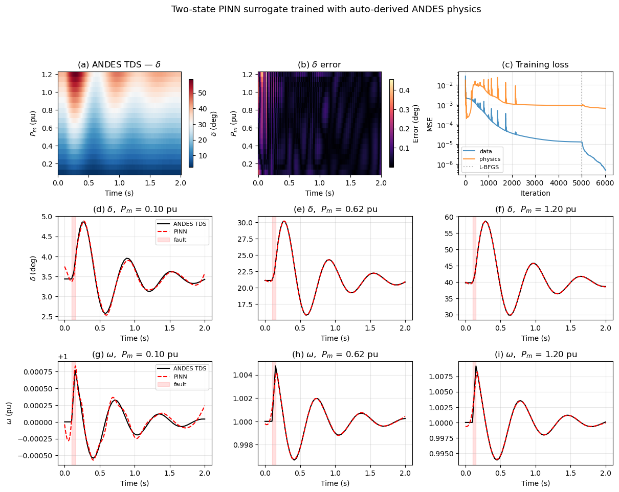
The two-state PINN achieves sub-degree accuracy for \(\delta\) and sub-0.002 pu accuracy for \(\omega\) across the full operating range, without any hand-coded physics. Both first-order ODEs from ANDES are enforced directly as the physics loss. The error is concentrated near the fault window where the ODE residuals are not enforced.
This pipeline generalizes to any ANDES model: calling prepare() on
a higher-order machine (e.g., GENROU with multiple differential states)
produces a larger set of symbolic equations that can be processed
through the same elimination and lambdification steps.
Extend This Example#
Higher-order models: replace GENCLS with GENROU to capture sub-transient dynamics and flux-decay effects in the surrogate.
Larger networks: parameterize the PINN over load levels or line impedances on multi-machine systems.
Fast contingency screening: once trained, the surrogate evaluates orders of magnitude faster than TDS, enabling real-time stability assessment.
Reinforcement learning: combine the surrogate with an RL agent for control design; see the RL Oscillation Damping on SMIB gallery example.
No output file found in the working directory.