Low-Inertia Frequency Stability

As inverter-based resources displace synchronous generators, the total rotational inertia of a power system declines. Since inverter-based resources do not inherently contribute inertial response, the system frequency becomes increasingly sensitive to generation-load imbalances. Two metrics characterize this degradation: the rate of change of frequency (RoCoF) immediately following a disturbance, and the frequency nadir, the minimum frequency reached before governor action arrests the decline.

This notebook quantifies the relationship between system inertia and frequency stability on the IEEE 14-bus system (5 GENROU generators with AVR and governor controls) by:

1. Scaling the inertia constants of all generators by a factor \(\alpha\) to emulate progressive renewable penetration.

2. Tripping the largest generator at each inertia level and recording the rotor speed transient.

3. Computing the center-of-inertia (COI) frequency and comparing RoCoF and nadir across scenarios.

Show code cell source

Hide code cell source

%matplotlib inline

import numpy as np
import pandas as pd
from matplotlib import pyplot as plt

import andes

andes.config_logger(stream_level=30)

System Setup

The IEEE 14-bus system contains five GENROU synchronous generators equipped with AVR exciters and turbine governors. The presence of these controllers produces well-damped transient responses that clearly illustrate the effect of inertia on frequency dynamics.

case_path = andes.get_case("ieee14/ieee14_full.xlsx")
ss_ref = andes.load(case_path)
ss_ref.PFlow.run()

gen_idxs = list(ss_ref.GENROU.idx.v)
gen_buses = list(ss_ref.GENROU.bus.v)
M_base = ss_ref.GENROU.M.v.copy()

gen_info = pd.DataFrame({"gen_idx": gen_idxs, "bus": gen_buses, "M": M_base})
gen_info.sort_values("M", ascending=False)

	gen_idx	bus	M
1	GENROU_2	2	13.0
3	GENROU_4	6	10.0
2	GENROU_3	3	10.0
4	GENROU_5	8	10.0
0	GENROU_1	1	8.0

Frequency Response Under Varying Inertia

The largest generator by inertia is tripped at \(t = 1\) s using a Toggle device. Seven inertia scaling factors from \(\alpha = 1.0\) down to \(\alpha = 0.15\) are simulated. The inertia constant \(M\) of every generator is scaled by \(\alpha\) before each time-domain run.

trip_idx = gen_idxs[int(np.argmax(M_base))]

inertia_scales = [1.0, 0.7, 0.5, 0.4, 0.3, 0.2, 0.15]
results = {}

for alpha in inertia_scales:
    ss = andes.load(case_path, setup=False)
    ss.add("Toggle", model="GENROU", dev=trip_idx, t=1.0)
    ss.setup()
    ss.config.warn_abnormal = 0
    ss.GENROU.M.v[:] = M_base * alpha

    ss.PFlow.run()
    ss.TDS.config.tf = 8
    ss.TDS.config.no_tqdm = 1
    ss.TDS.run()

    results[alpha] = ss.TDS.get_timeseries(ss.GENROU.omega)

COI Frequency After Generator Trip

The center-of-inertia (COI) frequency is computed as the inertia-weighted average of all generator rotor speeds:

\[f_\mathrm{COI} = \left(\sum_i \frac{M_i}{\sum_j M_j}\,\omega_i\right) \times 60 \;\text{Hz}\]

Since the swing equation relates \(M_i\,d\omega_i/dt\) to the power imbalance at each machine, the COI frequency directly reflects the aggregate generation-load mismatch following the disturbance.

Show code cell source

Hide code cell source

weights = M_base / M_base.sum()
cmap = plt.cm.RdYlBu

fig, ax = plt.subplots(figsize=(6, 4))

for i, (alpha, omega_df) in enumerate(results.items()):
    f_coi = (omega_df.values * weights).sum(axis=1) * 60
    color = cmap(i / (len(results) - 1))
    ax.plot(omega_df.index, f_coi, color=color, linewidth=1.8,
            label=f"$\\alpha$ = {alpha}")

ax.set_xlabel("Time [s]")
ax.set_ylabel("COI frequency [Hz]")
ax.set_title("IEEE 14-bus: frequency response after generator trip")
ax.legend(loc="lower right", fontsize=9, framealpha=0.9)
ax.set_xlim(0.5, 5.0)
ax.axhline(60.0, color="black", linewidth=0.4, alpha=0.3)

plt.tight_layout()

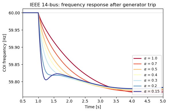
As the inertia scaling factor decreases from blue (\(\alpha = 1.0\)) to red (\(\alpha = 0.15\)), the initial rate of frequency decline steepens progressively. The curves fan out clearly in the first two seconds following the disturbance, and the well-damped oscillations produced by the AVR and governor controls confirm that the transient is dominated by the inertial response rather than by sustained electromechanical modes.

Quantitative Metrics

The RoCoF is estimated as the maximum absolute rate of frequency change within the first second after the disturbance. The nadir is the minimum COI frequency reached before governor action arrests the decline.

metrics = []
for alpha, omega_df in results.items():
    f_coi = (omega_df.values * weights).sum(axis=1) * 60
    t = omega_df.index.values

    nadir = f_coi[t > 1.0].min()

    post = (t >= 1.0) & (t <= 2.0)
    t_post, f_post = t[post], f_coi[post]
    rocof = np.max(np.abs(np.diff(f_post) / np.diff(t_post)))

    metrics.append({"α": alpha, "Nadir [Hz]": nadir, "RoCoF [Hz/s]": rocof})

metrics_df = pd.DataFrame(metrics).set_index("α")
metrics_df

	Nadir [Hz]	RoCoF [Hz/s]
α
1.00	59.767679	0.297080
0.70	59.771490	0.423739
0.50	59.775179	0.592006
0.40	59.776735	0.738667
0.30	59.777930	0.981922
0.20	59.778977	1.464048
0.15	59.779485	1.940406

RoCoF vs. Inertia Level

Show code cell source

Hide code cell source

fig, ax = plt.subplots(figsize=(6, 4))

ax.plot(metrics_df.index, metrics_df["RoCoF [Hz/s]"], "s-", color="tab:red",
        markersize=6)
ax.set_xlabel("Inertia scale factor $\\alpha$")
ax.set_ylabel("RoCoF [Hz/s]")
ax.set_title("Rate of change of frequency vs. inertia")
ax.invert_xaxis()

plt.tight_layout()

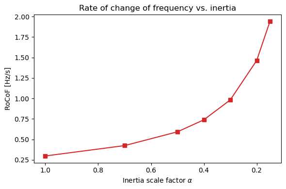
Reducing the system inertia monotonically increases the RoCoF following the generator trip. From \(\alpha = 1.0\) to \(\alpha = 0.15\), the RoCoF increases by approximately six times. Although the IEEE 14-bus system is small, the same qualitative behavior applies to larger interconnections: as synchronous generation is displaced by inverter-based resources without synthetic inertia, the system frequency becomes increasingly vulnerable to sudden imbalances.

Extend This Example

• Add synthetic inertia: install IBR models with frequency-watt droop (via REECA1) and compare the RoCoF improvement at low \(\alpha\).

• Vary the contingency size: trip different generators to study how disturbance magnitude interacts with inertia levels.

• Sweep inertia continuously: use a finer grid of \(\alpha\) values to trace the RoCoF curve more precisely.

• Add UFLS relays: implement under-frequency load shedding and observe the threshold at which it is triggered as inertia decreases.