2. First Simulation

This tutorial walks you through your first power system simulation using ANDES. By the end, you will have run power flow, time-domain simulation, and eigenvalue analysis on a test system. The entire workflow can be completed in about 5 minutes.

2.1. Import ANDES

Like other Python libraries, ANDES needs to be imported into an interactive Python environment before use. The config_logger function sets up the logging system that controls what messages ANDES displays during execution. Setting stream_level=20 corresponds to the INFO level, which shows normal operation messages without excessive detail.

# display plots in notebooks
%matplotlib inline

import andes

andes.config_logger(stream_level=20)

2.2. Load a Test Case

ANDES includes several built-in test cases that are useful for learning and validation. The andes.get_case() function returns the full path to a built-in case file, which can then be passed to andes.load() to create a System object.

In this tutorial, we use the Kundur two-area test system, a well-known benchmark for transient stability studies. This system contains four generators, two areas connected by weak tie-lines, and includes dynamic models for exciters and governors.

ss = andes.load(andes.get_case('kundur/kundur_full.xlsx'))

Working directory: "/home/docs/checkouts/readthedocs.org/user_builds/andes/checkouts/stable/docs/source/tutorials"
> Loaded generated Python code in "/home/docs/.andes/pycode".
Parsing input file "/home/docs/checkouts/readthedocs.org/user_builds/andes/envs/stable/lib/python3.11/site-packages/andes/cases/kundur/kundur_full.xlsx"...
Input file parsed in 0.0314 seconds.
Connectivity check completed in 0.0001 seconds.
-> System connectivity check results:
  No islanded bus detected.
  System is interconnected.
  Each island has a slack bus correctly defined and enabled.
System internal structure set up in 0.0209 seconds.

The variable ss is now an instance of the System class, which serves as the central container for all power system data, device models, and analysis routines. The naming convention ss (short for "system") is commonly used throughout ANDES examples and documentation. You can inspect the system by simply typing ss to see a summary of loaded models.

ss

<andes.system.facade.System at 0x774e122ebb10>

2.3. Run Power Flow

Before performing any dynamic simulation, you must first solve the power flow to establish a valid steady-state operating point. Power flow calculates the voltage magnitude and angle at each bus, as well as the active and reactive power flows throughout the network. ANDES uses the Newton-Raphson method, which typically converges within a few iterations for well-conditioned systems.

The power flow routine is accessed through ss.PFlow, and you run it by calling the run() method.

Note

In the PDF version of this documentation, detailed solver outputs are hidden to reduce repetition. To see the full outputs, refer to the online HTML documentation.

ss.PFlow.run()

-> Power flow calculation
           Numba: Off
   Sparse solver: KLU
 Solution method: NR method
Power flow initialized in 0.0039 seconds.
0: |F(x)| = 14.9282832
1: |F(x)| = 3.608627841
2: |F(x)| = 0.1701107882
3: |F(x)| = 0.002038626956
4: |F(x)| = 3.745103977e-07
Converged in 5 iterations in 0.0026 seconds.
Report saved to "kundur_full_out.txt" in 0.0009 seconds.

True

After the power flow converges, you can access the solved values through the model objects. For example, the bus voltage magnitudes are stored in ss.Bus.v.v, where the first v refers to the voltage variable and the second v accesses its numerical value array.

ss.Bus.v.v

array([1.        , 1.        , 1.        , 1.        , 0.98337472,
       0.96908586, 0.95621812, 0.95400019, 0.96856366, 0.98377143])

2.4. Run Time-Domain Simulation

Time-domain simulation (TDS) solves the differential-algebraic equations (DAEs) that govern power system dynamics. This allows you to study how the system responds to disturbances such as faults, line trips, or generator outages. ANDES uses the implicit trapezoidal method for numerical integration, which provides good accuracy and numerical stability.

Before running TDS, you can configure simulation parameters through ss.TDS.config. The most commonly adjusted parameter is tf, which sets the simulation end time in seconds. The Kundur test case includes a pre-defined line trip disturbance at t=2 seconds, so we simulate for 10 seconds to observe the system response.

ss.TDS.config.tf = 10
ss.TDS.run()

DAE compaction: removed 5 algebraic variable slots (m: 149 -> 144)
Initialization for dynamics completed in 0.0162 seconds.
Initialization was successful.
<Toggle 1>: Line.Line_8 status changed to 0 at t=2.0 sec.
Simulation to t=10.00 sec completed in 0.5468 seconds.
Outputs to "kundur_full_out.lst" and "kundur_full_out.npz".
Outputs written in 0.0144 seconds.

True

The simulation output shows the progress as time advances. When the line trips at t=2s, the generators experience a sudden change in loading conditions, causing their rotors to oscillate as they seek a new equilibrium point.

2.5. Plot Results

ANDES provides a built-in plotting interface through ss.TDS.plt that makes it easy to visualize simulation results. The plot() method accepts a variable object and automatically retrieves its time series data.

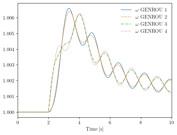
To see the dynamic response, we plot the generator rotor speeds (omega). In a stable system, the speeds should oscillate after the disturbance and eventually settle to a new steady-state value. The GENROU model represents round-rotor synchronous generators, which are the four machines in this test system.

ss.TDS.plt.plot(ss.GENROU.omega)

Using LaTeX for rendering. If an error occurs:
a) If you are using `andes plot`, disable with option "-d",
b) If you are using `plot()`, set "latex=False".

(<Figure size 640x480 with 1 Axes>, <Axes: xlabel='Time [s]'>)

The plot shows the characteristic inter-area oscillations of the Kundur two-area system. Generators in the same area tend to swing together, while generators in different areas swing against each other. This oscillatory mode is a key concern in power system stability analysis.

2.6. Run Eigenvalue Analysis

Eigenvalue analysis examines small-signal stability by linearizing the system equations around the operating point and computing the eigenvalues of the state matrix. The location of eigenvalues in the complex plane indicates system stability: eigenvalues with negative real parts correspond to stable modes, while those with positive real parts indicate instability.

For eigenvalue analysis, we load a fresh system instance because TDS modifies internal states during simulation. After running power flow to establish the operating point, we call ss2.EIG.run() to perform the eigenvalue calculation.

ss2 = andes.load(andes.get_case('kundur/kundur_full.xlsx'))
ss2.PFlow.run()
ss2.EIG.run()

Working directory: "/home/docs/checkouts/readthedocs.org/user_builds/andes/checkouts/stable/docs/source/tutorials"
> Reloaded generated Python code of module "pycode".
Parsing input file "/home/docs/checkouts/readthedocs.org/user_builds/andes/envs/stable/lib/python3.11/site-packages/andes/cases/kundur/kundur_full.xlsx"...
Input file parsed in 0.0297 seconds.
Connectivity check completed in 0.0001 seconds.
-> System connectivity check results:
  No islanded bus detected.
  System is interconnected.
  Each island has a slack bus correctly defined and enabled.
System internal structure set up in 0.0194 seconds.

-> Power flow calculation
           Numba: Off
   Sparse solver: KLU
 Solution method: NR method
Power flow initialized in 0.0030 seconds.
0: |F(x)| = 14.9282832
1: |F(x)| = 3.608627841
2: |F(x)| = 0.1701107882
3: |F(x)| = 0.002038626956
4: |F(x)| = 3.745103977e-07
Converged in 5 iterations in 0.0024 seconds.
Report saved to "kundur_full_out.txt" in 0.0005 seconds.
DAE compaction: removed 5 algebraic variable slots (m: 149 -> 144)
Initialization for dynamics completed in 0.0151 seconds.
Initialization was successful.

-> Eigenvalue Analysis:
  Positive       0
  Zeros          1
  Negative      52
Eigenvalue analysis finished in 0.0026 seconds.
Report saved to "kundur_full_eig.txt".

True

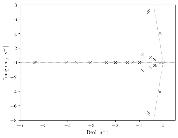
The eigenvalue results can be visualized on the s-plane using the plot() method. Each point represents an eigenvalue, with the x-axis showing the real part (damping) and the y-axis showing the imaginary part (oscillation frequency).

ss2.EIG.plot()

(<Figure size 640x480 with 1 Axes>,
 <Axes: xlabel='Real [$s^{-1}$]', ylabel='Imaginary [$s^{-1}$]'>)

2.7. Key Concepts

The following table summarizes the main components you have encountered in this tutorial.

Concept	Description
System	Central container that holds all models, parameters, and analysis routines
PFlow	Power flow routine using Newton-Raphson iteration
TDS	Time-domain simulation using implicit trapezoidal integration
EIG	Eigenvalue analysis for small-signal stability assessment
Models	Device representations such as Bus, PQ, GENROU, TGOV1, EXDC2

2.8. Using the Command Line

In addition to the Python interface, ANDES provides a command-line interface (CLI) for running simulations without writing code. This is convenient for batch processing or quick analyses. The following examples demonstrate common CLI usage patterns.

# Run power flow (default routine)
andes run ieee14.json

# Run time-domain simulation
andes run kundur_full.xlsx -r tds

# Run eigenvalue analysis
andes run kundur_full.xlsx -r eig

# Plot results from output files
andes plot kundur_full_out.lst 0 5 6 7 8

The -r flag specifies which routine to run. Without it, ANDES runs power flow by default. Output files are automatically generated with the case name as a prefix.

2.9. Cleanup

Simulations generate output files including result data (.npz), variable listings (.lst), and reports (.txt). The following command removes these files from the current directory.

!andes misc -C

"/home/docs/checkouts/readthedocs.org/user_builds/andes/checkouts/stable/docs/source/tutorials/kundur_full_eig.txt" removed.
"/home/docs/checkouts/readthedocs.org/user_builds/andes/checkouts/stable/docs/source/tutorials/kundur_full_out.txt" removed.
"/home/docs/checkouts/readthedocs.org/user_builds/andes/checkouts/stable/docs/source/tutorials/kundur_full_out.lst" removed.
"/home/docs/checkouts/readthedocs.org/user_builds/andes/checkouts/stable/docs/source/tutorials/kundur_full_out.npz" removed.

2.10. Next Steps

Now that you have completed your first simulation, you can explore more advanced topics:

• Power Flow Analysis - Detailed power flow analysis and troubleshooting

• Time-Domain Simulation - Adding disturbances and configuring simulations

• Data and File Formats - Loading different file formats and modifying parameters