7. Eigenvalue Analysis#
Eigenvalue analysis (also called small-signal stability analysis) examines how a power system responds to small perturbations around its operating point. By linearizing the nonlinear differential-algebraic equations and computing the eigenvalues of the resulting state matrix, we can determine whether the system is stable and identify the oscillatory modes that dominate its dynamic behavior.
This analysis is fundamental to understanding inter-area oscillations, local plant modes, and control interactions. The location of eigenvalues in the complex plane tells us about stability: eigenvalues with negative real parts indicate stable modes (perturbations decay), while eigenvalues with positive real parts indicate unstable modes (perturbations grow). The imaginary part relates to the oscillation frequency.
This tutorial demonstrates how to run eigenvalue analysis in ANDES and interpret the results.
7.1. Setup#
%matplotlib inline

import numpy as np
import andes

andes.config_logger(stream_level=20)
7.2. Running Eigenvalue Analysis#
Eigenvalue analysis requires an established operating point, so ANDES automatically runs power flow before computing eigenvalues. The simplest way to run eigenvalue analysis is to pass routine='eig' to andes.run(), which loads the case, runs power flow, and then performs the eigenvalue calculation in a single step.
case_path = andes.get_case('kundur/kundur_full.xlsx')
ss = andes.run(case_path, routine='eig')
Working directory: "/home/docs/checkouts/readthedocs.org/user_builds/andes/checkouts/stable/docs/source/tutorials"
> Loaded generated Python code in "/home/docs/.andes/pycode".
Parsing input file "/home/docs/checkouts/readthedocs.org/user_builds/andes/envs/stable/lib/python3.11/site-packages/andes/cases/kundur/kundur_full.xlsx"...
Input file parsed in 0.0313 seconds.
Connectivity check completed in 0.0001 seconds.
-> System connectivity check results:
  No islanded bus detected.
  System is interconnected.
  Each island has a slack bus correctly defined and enabled.
System internal structure set up in 0.0205 seconds.

-> Power flow calculation
           Numba: Off
   Sparse solver: KLU
 Solution method: NR method
Power flow initialized in 0.0031 seconds.
0: |F(x)| = 14.9282832
1: |F(x)| = 3.608627841
2: |F(x)| = 0.1701107882
3: |F(x)| = 0.002038626956
4: |F(x)| = 3.745103977e-07
Converged in 5 iterations in 0.0025 seconds.
Report saved to "kundur_full_out.txt" in 0.0008 seconds.
DAE compaction: removed 5 algebraic variable slots (m: 149 -> 144)
Initialization for dynamics completed in 0.0152 seconds.
Initialization was successful.

-> Eigenvalue Analysis:
  Positive       0
  Zeros          1
  Negative      52
Eigenvalue analysis finished in 0.0018 seconds.
Report saved to "kundur_full_eig.txt".
-> Single process finished in 0.6308 seconds.
The output shows that the system has 52 negative eigenvalues, 1 zero eigenvalue, and 0 positive eigenvalues. The zero eigenvalue is expected and corresponds to the rotor angle reference (absolute angles are not observable, only relative angles matter). The absence of positive eigenvalues indicates that the system is stable for small perturbations.
Alternatively, you can run eigenvalue analysis step by step after loading the system:
# Step-by-step approach
ss2 = andes.load(andes.get_case('kundur/kundur_full.xlsx'))
ss2.PFlow.run()
ss2.EIG.run()
Working directory: "/home/docs/checkouts/readthedocs.org/user_builds/andes/checkouts/stable/docs/source/tutorials"
> Reloaded generated Python code of module "pycode".
Parsing input file "/home/docs/checkouts/readthedocs.org/user_builds/andes/envs/stable/lib/python3.11/site-packages/andes/cases/kundur/kundur_full.xlsx"...
Input file parsed in 0.0305 seconds.
Connectivity check completed in 0.0001 seconds.
-> System connectivity check results:
  No islanded bus detected.
  System is interconnected.
  Each island has a slack bus correctly defined and enabled.
System internal structure set up in 0.0189 seconds.

-> Power flow calculation
           Numba: Off
   Sparse solver: KLU
 Solution method: NR method
Power flow initialized in 0.0030 seconds.
0: |F(x)| = 14.9282832
1: |F(x)| = 3.608627841
2: |F(x)| = 0.1701107882
3: |F(x)| = 0.002038626956
4: |F(x)| = 3.745103977e-07
Converged in 5 iterations in 0.0024 seconds.
Report saved to "kundur_full_out.txt" in 0.0005 seconds.
DAE compaction: removed 5 algebraic variable slots (m: 149 -> 144)
Initialization for dynamics completed in 0.0149 seconds.
Initialization was successful.

-> Eigenvalue Analysis:
  Positive       0
  Zeros          1
  Negative      52
Eigenvalue analysis finished in 0.0015 seconds.
Report saved to "kundur_full_eig.txt".
True
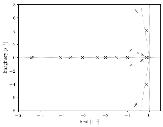
7.3. Plotting Eigenvalues on the S-Plane#
The eigenvalue results are most easily interpreted through visualization. The ss.EIG.plot() method creates an s-plane plot where the x-axis represents the real part (damping) and the y-axis represents the imaginary part (oscillation frequency in rad/s).
ss.EIG.plot()
(<Figure size 640x480 with 1 Axes>,
 <Axes: xlabel='Real [$s^{-1}$]', ylabel='Imaginary [$s^{-1}$]'>)
In the plot, eigenvalues appearing on the left half of the plane (negative real part) represent stable modes. Those closer to the imaginary axis are less damped and will decay slowly after a disturbance. Eigenvalues with larger imaginary parts correspond to higher-frequency oscillations.
For the Kundur two-area system, you can identify several types of modes:
Modes near the origin with small imaginary parts are often inter-area oscillation modes
Modes farther from the origin typically correspond to local generator modes and exciter/governor dynamics
Real eigenvalues (on the real axis) represent non-oscillatory modes
7.4. Eigenvalue Report#
ANDES generates a detailed report file (*_eig.txt) containing the computed eigenvalues, their damping ratios, and frequencies. This report is useful for detailed analysis and documentation.
with open('kundur_full_eig.txt', 'r') as f:
    content = f.read()
    # Print first 2000 characters to see the structure
    print(content[:2000])
ANDES 2.0.0
Copyright (C) 2015-2026 Hantao Cui

ANDES comes with ABSOLUTELY NO WARRANTY
Case file: /home/docs/checkouts/readthedocs.org/user_builds/andes/envs/stable/lib/python3.11/site-packages/andes/cases/kundur/kundur_full.xlsx
Report time: 03/12/2026 05:07:07 PM

Power flow converged in 5 iterations.
Flat-start: No


EIGENVALUE ANALYSIS REPORT

Positives
Zeros
Negatives

STATISTICS
                     Most Associated              Real             Imag.      Damped Freq.         Frequency       Damping [%]

#1                      LL_x EXDC2 1                -1                 0                 0                 0                 0
#2                      LL_x EXDC2 2                -1                 0                 0                 0                 0
#3                      LL_x EXDC2 3                -1                 0                 0                 0                 0
#4                      LL_x EXDC2 4                -1                 0                 0                 0                 0
#5                      LS_y EXDC2 1           -49.541                 0                 0                 0                 0
#6                      LS_y EXDC2 1           -49.526                 0                 0                 0                 0
#7                      LA_y EXDC2 3           -49.199            0.4645          0.073927            7.8306            99.996
#8                      LA_y EXDC2 3           -49.199           -0.4645          0.073927            7.8306            99.996
#9                      LS_y EXDC2 1           -49.203           0.34143           0.05434            7.8312            99.998
#10                     LS_y EXDC2 1           -49.203          -0.34143           0.05434            7.8312            99.998
#11                     LA_y EXDC2 1            -48.88                 0                 0                 0                 0
#12
7.5. Parameter Sweeps and Root Loci#
One of the most powerful applications of eigenvalue analysis is studying how eigenvalues move as system parameters change. This root locus analysis helps identify parameter ranges that maintain stability and shows which modes are most sensitive to parameter variations.
The ss.EIG.sweep() method automates this process by repeatedly computing eigenvalues for different parameter values. In this example, we study how the exciter gain KA of the first EXDC2 exciter affects system stability by varying it from 20 to 200.
# Sweep KA from 20 to 200 in 10 steps
ret = ss.EIG.sweep(ss.EXDC2.KA, 1, np.linspace(20, 200, 10))
The sweep() method returns a dictionary containing the eigenvalues computed at each parameter value. We can then visualize how specific eigenvalues move using plot_root_loci().
The following plot shows eigenvalues 30 through 50 (zero-indexed). The marker size increases with the parameter value, so larger markers correspond to higher exciter gains. This allows you to track the trajectory of each eigenvalue as the parameter increases.
ss.EIG.plot_root_loci(ret, range(30, 51), left=-3, ymax=4, ymin=-4)
(<Figure size 640x480 with 1 Axes>,
 <Axes: xlabel='Real [$s^{-1}$]', ylabel='Imaginary [$s^{-1}$]'>)
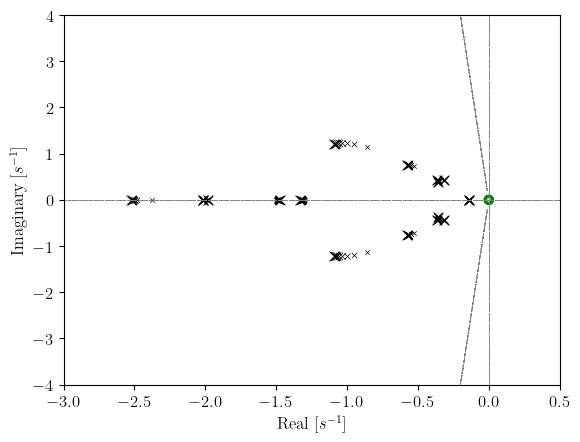
The root locus plot reveals how increasing the exciter gain affects system modes. If eigenvalues move toward the right (toward the imaginary axis or beyond), the system becomes less stable or potentially unstable. If they move left, the system becomes more damped.
This type of analysis is invaluable for tuning controller parameters. By observing the root loci, you can identify the parameter range that provides acceptable damping while avoiding instability.
7.6. Cleanup#
!andes misc -C
"/home/docs/checkouts/readthedocs.org/user_builds/andes/checkouts/stable/docs/source/tutorials/kundur_full_eig.txt" removed.
"/home/docs/checkouts/readthedocs.org/user_builds/andes/checkouts/stable/docs/source/tutorials/kundur_full_out.txt" removed.
7.7. Next Steps#
Parameter Sweeps and Batch Processing - Batch simulations for sensitivity studies
Contingency Analysis - N-1 contingency screening
Dynamic Control and Setpoint Changes - Runtime parameter control