13. Continuation Power Flow

Standard power flow computes the operating point at a given loading level, but it cannot determine how far the system is from voltage collapse. Continuation power flow (CPF) answers this question by tracing the relationship between loading and bus voltages, known as the nose curve or PV curve, from the base case up to and beyond the maximum loadability point.

The CPF uses a predictor-corrector method with a continuation parameter \(\lambda\) that interpolates between the base case (\(\lambda=0\)) and a target loading condition (\(\lambda=1\)):

\[p(\lambda) = p_{\text{base}} + \lambda \cdot (p_{\text{target}} - p_{\text{base}})\]

At each step, a tangent predictor estimates the next point on the curve, and an augmented Newton-Raphson corrector refines it. The maximum \(\lambda\) achieved gives the steady-state loadability limit, the point beyond which no power flow solution exists.

This tutorial covers running CPF in ANDES, interpreting results, plotting PV curves, QV curve analysis for reactive power margins, selecting parameterization methods, and specifying custom loading targets.

%matplotlib inline

# Reduce logging verbosity for PDF builds
import os
if os.environ.get('SPHINX_BUILD_PDF'):
    import andes
    _orig_config_logger = andes.config_logger
    def _quiet_logger(stream_level=20, *args, **kwargs):
        stream_level = max(stream_level, 30)
        return _orig_config_logger(stream_level, *args, **kwargs)
    andes.config_logger = _quiet_logger

13.1. Setup

CPF requires a converged power flow as its starting point. We load the IEEE 14-bus system and run power flow first.

import numpy as np
import andes
from matplotlib import pyplot as plt

andes.config_logger(stream_level=20)

ss = andes.load(andes.get_case('ieee14/ieee14.json'))
ss.PFlow.run()

Working directory: "/home/docs/checkouts/readthedocs.org/user_builds/andes/checkouts/stable/docs/source/tutorials"
> Loaded generated Python code in "/home/docs/.andes/pycode".
Parsing input file "/home/docs/checkouts/readthedocs.org/user_builds/andes/envs/stable/lib/python3.11/site-packages/andes/cases/ieee14/ieee14.json"...
Input file parsed in 0.0020 seconds.
Connectivity check completed in 0.0001 seconds.
-> System connectivity check results:
  No islanded bus detected.
  System is interconnected.
  Each island has a slack bus correctly defined and enabled.
System internal structure set up in 0.0198 seconds.

-> Power flow calculation
           Numba: Off
   Sparse solver: KLU
 Solution method: NR method
Power flow initialized in 0.0033 seconds.
0: |F(x)| = 0.5605182134
1: |F(x)| = 0.006202200332
2: |F(x)| = 5.819382827e-06
3: |F(x)| = 6.957087684e-12
Converged in 4 iterations in 0.0022 seconds.
Report saved to "ieee14_out.txt" in 0.0010 seconds.

True

13.2. Running CPF

The simplest way to run CPF is to specify a uniform load scaling factor. A load_scale of 2.0 means the target loading is twice the base case: all PQ loads and PV generation are scaled proportionally. The CPF traces the nose curve from \(\lambda=0\) (base case) toward \(\lambda=1\) (target), and beyond if the system can sustain it.

ss.CPF.run(load_scale=2.0)

-> Continuation Power Flow
Parameterization: pseudo_arclength
       Step size: 0.1
   Adaptive step: On
         Stop at: NOSE
Nose detected at step 16, lambda=3.167739

-> CPF Report
       Converged: True
           Steps: 17
      Max lambda: 3.258046
     Termination: Nose point at lambda=3.258046
CPF completed in 17 steps in 0.0374 seconds. max lambda = 3.258046

True

The CPF report shows the number of continuation steps, the maximum \(\lambda\) reached (the loadability limit), and the termination reason. A max_lam greater than 1.0 means the system can sustain the full target loading; the nose point occurs at some higher loading level.

The run() method returns True if the CPF terminated as expected for the requested stop_at mode:

• stop_at='NOSE' (default): terminates at the nose point (maximum loadability)

• stop_at='FULL': traces both the upper and lower branches, returning to \(\lambda=0\)

• stop_at=float: terminates when \(\lambda\) reaches the specified value

The key results are stored as NumPy arrays:

Attribute	Shape	Description
ss.CPF.lam	(npoints,)	Continuation parameter \(\lambda\) at each step
ss.CPF.V	(nbus, npoints)	Bus voltage magnitudes at each step
ss.CPF.theta	(nbus, npoints)	Bus voltage angles at each step
ss.CPF.max_lam	scalar	Maximum \(\lambda\) (loadability limit)
ss.CPF.steps	(npoints-1,)	Step sizes used at each continuation step

ss.CPF.max_lam

3.2580458612253804

13.3. Plotting the Nose Curve

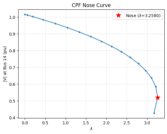
The PV curve reveals how bus voltages change with loading. Weak buses, those with the steepest voltage decline, are the most vulnerable to voltage collapse. The built-in plot() method creates a PV curve for a specified bus, with the nose point marked.

fig, ax = ss.CPF.plot(bus_idx=14, show=False)
plt.show()

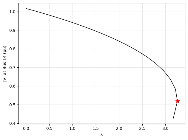
The V, lam, and theta arrays can be used directly for custom analysis. The following example extracts the nose-point data, identifies the weakest bus, and plots a publication-quality PV curve.

lam = ss.CPF.lam
nose = np.argmax(lam)

# Weakest bus = largest voltage drop from base to nose.
weak = np.argmax(ss.CPF.V[:, 0] - ss.CPF.V[:, nose])

fig, ax = plt.subplots()
ax.plot(lam, ss.CPF.V[weak, :], 'k-', linewidth=1.2)
ax.plot(lam[nose], ss.CPF.V[weak, nose], 'r*', markersize=10)
ax.set_xlabel(r'$\lambda$')
ax.set_ylabel(f'|V| at Bus {ss.Bus.idx.v[weak]} (pu)')
ax.grid(True, alpha=0.3)
fig.tight_layout()
plt.show()

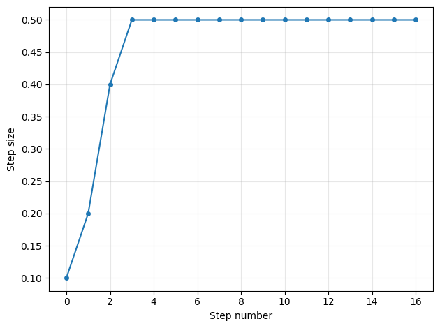
fig, ax = plt.subplots()
ax.plot(range(len(ss.CPF.steps)), ss.CPF.steps, 'o-', markersize=4)
ax.set_xlabel('Step number')
ax.set_ylabel('Step size')
ax.grid(True, alpha=0.3)
fig.tight_layout()
plt.show()

13.4. Parameterization Methods

The parameterization determines how the corrector constrains the solution at each step. Different methods have different trade-offs near the nose point, where the standard power flow Jacobian becomes singular.

ANDES provides three parameterization methods:

Method	Description	Behavior at nose
pseudo_arclength	Constrains the step along the tangent direction	Most robust; can trace through the nose point
arclength	Constrains the Euclidean distance from the previous point	Traces the full curve; may take more steps
natural	Fixes \(\lambda\) increment directly	Simplest; fails at the nose point

Pseudo arc-length is the default because it handles the nose point most reliably. Natural parameterization is the simplest conceptually but becomes singular exactly at the loadability limit, making it unable to trace the lower branch of the PV curve.

The parameterization is selected through the configuration before running CPF.

# reload to get a fresh system
ss2 = andes.load(andes.get_case('ieee14/ieee14.json'))
ss2.PFlow.run()

ss2.CPF.config.parameterization = 'arclength'
ss2.CPF.run(load_scale=2.0)

Working directory: "/home/docs/checkouts/readthedocs.org/user_builds/andes/checkouts/stable/docs/source/tutorials"
> Reloaded generated Python code of module "pycode".
Parsing input file "/home/docs/checkouts/readthedocs.org/user_builds/andes/envs/stable/lib/python3.11/site-packages/andes/cases/ieee14/ieee14.json"...
Input file parsed in 0.0019 seconds.
Connectivity check completed in 0.0001 seconds.
-> System connectivity check results:
  No islanded bus detected.
  System is interconnected.
  Each island has a slack bus correctly defined and enabled.
System internal structure set up in 0.0190 seconds.

-> Power flow calculation
           Numba: Off
   Sparse solver: KLU
 Solution method: NR method
Power flow initialized in 0.0032 seconds.
0: |F(x)| = 0.5605182134
1: |F(x)| = 0.006202200332
2: |F(x)| = 5.819382827e-06
3: |F(x)| = 6.957087684e-12
Converged in 4 iterations in 0.0020 seconds.
Report saved to "ieee14_out.txt" in 0.0006 seconds.

-> Continuation Power Flow
Parameterization: arclength
       Step size: 0.1
   Adaptive step: On
         Stop at: NOSE
Nose detected at step 16, lambda=3.175750

-> CPF Report
       Converged: True
           Steps: 17
      Max lambda: 3.258050
     Termination: Nose point at lambda=3.258050
CPF completed in 17 steps in 0.0384 seconds. max lambda = 3.258050

True

ss2.CPF.max_lam

3.2580499020258302

All three methods should agree on the loadability limit to within a few percent, since they trace the same underlying curve. The differences arise from how finely they sample the curve near the nose.

13.5. Termination Control

By default, CPF terminates at the nose point (stop_at='NOSE'). In some analyses, it is useful to stop at a specific loading level instead, for example, to find the voltage profile at 1.5 times the base-case loading. Setting stop_at to a float value causes CPF to terminate when \(\lambda\) reaches that value, with the final step sized to land exactly on the target.

ss3 = andes.load(andes.get_case('ieee14/ieee14.json'))
ss3.PFlow.run()

ss3.CPF.config.stop_at = 1.5
ss3.CPF.run(load_scale=2.0)

Working directory: "/home/docs/checkouts/readthedocs.org/user_builds/andes/checkouts/stable/docs/source/tutorials"
> Reloaded generated Python code of module "pycode".
Parsing input file "/home/docs/checkouts/readthedocs.org/user_builds/andes/envs/stable/lib/python3.11/site-packages/andes/cases/ieee14/ieee14.json"...
Input file parsed in 0.0019 seconds.
Connectivity check completed in 0.0001 seconds.
-> System connectivity check results:
  No islanded bus detected.
  System is interconnected.
  Each island has a slack bus correctly defined and enabled.
System internal structure set up in 0.0186 seconds.

-> Power flow calculation
           Numba: Off
   Sparse solver: KLU
 Solution method: NR method
Power flow initialized in 0.0032 seconds.
0: |F(x)| = 0.5605182134
1: |F(x)| = 0.006202200332
2: |F(x)| = 5.819382827e-06
3: |F(x)| = 6.957087684e-12
Converged in 4 iterations in 0.0019 seconds.
Report saved to "ieee14_out.txt" in 0.0006 seconds.

-> Continuation Power Flow
Parameterization: pseudo_arclength
       Step size: 0.1
   Adaptive step: On
         Stop at: 1.5

-> CPF Report
       Converged: True
           Steps: 8
      Max lambda: 1.500000
     Termination: Reached target lambda=1.5
CPF completed in 8 steps in 0.0152 seconds. max lambda = 1.500000

True

ss3.CPF.lam[-1]

np.float64(1.5)

The final \(\lambda\) value is exactly the requested target (to within solver tolerance).

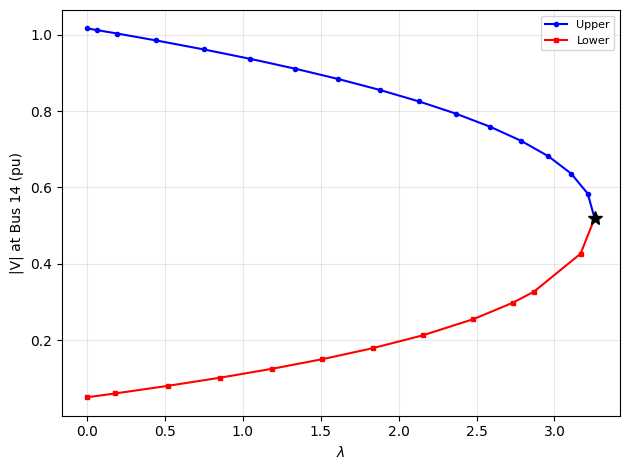
13.6. Full Curve Tracing (Upper and Lower Branches)

Setting stop_at='FULL' traces the complete nose curve: the upper branch from \(\lambda=0\) to the nose, then the lower (unstable) branch back down to \(\lambda=0\). At the nose point, the continuation detects the fold bifurcation and automatically switches to the lower branch. The lower branch represents unstable equilibrium points that are physically unrealizable but are important for voltage stability analysis.

The lower branch voltages are significantly below the upper branch at the same loading level. At \(\lambda=0\) on the lower branch, the bus voltages represent the low-voltage solution of the base-case power flow equations.

ss_full = andes.load(andes.get_case('ieee14/ieee14.json'))
ss_full.PFlow.run()

ss_full.CPF.config.stop_at = 'FULL'
ss_full.CPF.run(load_scale=2.0)

Working directory: "/home/docs/checkouts/readthedocs.org/user_builds/andes/checkouts/stable/docs/source/tutorials"
> Reloaded generated Python code of module "pycode".
Parsing input file "/home/docs/checkouts/readthedocs.org/user_builds/andes/envs/stable/lib/python3.11/site-packages/andes/cases/ieee14/ieee14.json"...
Input file parsed in 0.0021 seconds.
Connectivity check completed in 0.0001 seconds.
-> System connectivity check results:
  No islanded bus detected.
  System is interconnected.
  Each island has a slack bus correctly defined and enabled.
System internal structure set up in 0.0206 seconds.

-> Power flow calculation
           Numba: Off
   Sparse solver: KLU
 Solution method: NR method
Power flow initialized in 0.0035 seconds.
0: |F(x)| = 0.5605182134
1: |F(x)| = 0.006202200332
2: |F(x)| = 5.819382827e-06
3: |F(x)| = 6.957087684e-12
Converged in 4 iterations in 0.0020 seconds.
Report saved to "ieee14_out.txt" in 0.0006 seconds.

-> Continuation Power Flow
Parameterization: pseudo_arclength
       Step size: 0.1
   Adaptive step: On
         Stop at: FULL
Nose detected at step 16, lambda=3.167739

-> CPF Report
       Converged: True
           Steps: 28
      Max lambda: 3.258046
     Termination: Full curve traced (returned to lambda=0)
CPF completed in 28 steps in 0.0620 seconds. max lambda = 3.258046

True

lam = ss_full.CPF.lam
nose = np.argmax(lam)
weak = np.argmax(ss_full.CPF.V[:, 0] - ss_full.CPF.V[:, nose])

fig, ax = plt.subplots()
ax.plot(lam[:nose+1], ss_full.CPF.V[weak, :nose+1], 'b-o', markersize=3, label='Upper')
ax.plot(lam[nose:], ss_full.CPF.V[weak, nose:], 'r-s', markersize=3, label='Lower')
ax.plot(lam[nose], ss_full.CPF.V[weak, nose], 'k*', markersize=10)
ax.set_xlabel(r'$\lambda$')
ax.set_ylabel(f'|V| at Bus {ss_full.Bus.idx.v[weak]} (pu)')
ax.legend(fontsize=8)
ax.grid(True, alpha=0.3)
fig.tight_layout()
plt.show()

13.7. Per-Device Loading Targets

Uniform load scaling is the most common use case, but real planning studies often involve non-uniform load growth. For example, one area may grow faster than another. The p0_target and q0_target arguments accept per-device arrays that specify the target active and reactive power for each PQ load. Similarly, pg_target specifies the target generation for each PV generator.

The continuation parameter \(\lambda\) then interpolates between the base-case values and these per-device targets.

ss4 = andes.load(andes.get_case('ieee14/ieee14.json'))
ss4.PFlow.run()

# Double the load on the first 5 PQ buses, keep the rest unchanged
p0_base = ss4.PQ.p0.v.copy()
q0_base = ss4.PQ.q0.v.copy()

p0_target = p0_base.copy()
q0_target = q0_base.copy()
p0_target[:5] = p0_base[:5] * 3.0
q0_target[:5] = q0_base[:5] * 3.0

ss4.CPF.run(p0_target=p0_target, q0_target=q0_target)

Working directory: "/home/docs/checkouts/readthedocs.org/user_builds/andes/checkouts/stable/docs/source/tutorials"
> Reloaded generated Python code of module "pycode".
Parsing input file "/home/docs/checkouts/readthedocs.org/user_builds/andes/envs/stable/lib/python3.11/site-packages/andes/cases/ieee14/ieee14.json"...
Input file parsed in 0.0020 seconds.
Connectivity check completed in 0.0001 seconds.
-> System connectivity check results:
  No islanded bus detected.
  System is interconnected.
  Each island has a slack bus correctly defined and enabled.
System internal structure set up in 0.0187 seconds.

-> Power flow calculation
           Numba: Off
   Sparse solver: KLU
 Solution method: NR method
Power flow initialized in 0.0032 seconds.
0: |F(x)| = 0.5605182134
1: |F(x)| = 0.006202200332
2: |F(x)| = 5.819382827e-06
3: |F(x)| = 6.957087684e-12
Converged in 4 iterations in 0.0020 seconds.
Report saved to "ieee14_out.txt" in 0.0006 seconds.

-> Continuation Power Flow
Parameterization: pseudo_arclength
       Step size: 0.1
   Adaptive step: On
         Stop at: NOSE
Nose detected at step 56, lambda=3.516561

-> CPF Report
       Converged: True
           Steps: 57
      Max lambda: 3.517463
     Termination: Nose point at lambda=3.517463
CPF completed in 57 steps in 0.0992 seconds. max lambda = 3.517463

True

ss4.CPF.max_lam

3.5174627656369064

13.8. QV Curve Analysis

A QV curve shows the reactive power required to maintain a given voltage at a specific bus. The nose of the QV curve gives the reactive power margin, the additional reactive power absorption the bus can sustain before voltage collapse. While the PV curve parameterizes active power, the QV curve fixes active power everywhere and varies only reactive power at the target bus.

The run_qv() method builds the appropriate continuation target internally and delegates to the CPF engine. The q_range argument specifies the total reactive power sweep range in per-unit on the system base.

ss_qv = andes.load(andes.get_case('ieee14/ieee14.json'))
ss_qv.PFlow.run()

ss_qv.CPF.run_qv(bus_idx=14, q_range=3.0)

Working directory: "/home/docs/checkouts/readthedocs.org/user_builds/andes/checkouts/stable/docs/source/tutorials"
> Reloaded generated Python code of module "pycode".
Parsing input file "/home/docs/checkouts/readthedocs.org/user_builds/andes/envs/stable/lib/python3.11/site-packages/andes/cases/ieee14/ieee14.json"...
Input file parsed in 0.0020 seconds.
Connectivity check completed in 0.0001 seconds.
-> System connectivity check results:
  No islanded bus detected.
  System is interconnected.
  Each island has a slack bus correctly defined and enabled.
System internal structure set up in 0.0187 seconds.

-> Power flow calculation
           Numba: Off
   Sparse solver: KLU
 Solution method: NR method
Power flow initialized in 0.0032 seconds.
0: |F(x)| = 0.5605182134
1: |F(x)| = 0.006202200332
2: |F(x)| = 5.819382827e-06
3: |F(x)| = 6.957087684e-12
Converged in 4 iterations in 0.0021 seconds.
Report saved to "ieee14_out.txt" in 0.0006 seconds.

-> Continuation Power Flow
Parameterization: pseudo_arclength
       Step size: 0.1
   Adaptive step: On
         Stop at: NOSE
Nose detected at step 5, lambda=0.346459

-> CPF Report
       Converged: True
           Steps: 6
      Max lambda: 0.359814
     Termination: Nose point at lambda=0.359814
CPF completed in 6 steps in 0.0131 seconds. max lambda = 0.359814

True

fig, ax = ss_qv.CPF.plot_qv(show=False)
fig.tight_layout()
plt.show()

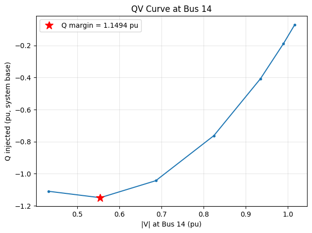
The QV curve results are stored in qv_q (reactive power in load convention) and qv_v (voltage magnitude), both 1-D arrays aligned with lam. The plot_qv() method negates qv_q to follow the standard convention where positive Q represents injection (capacitive support). The red star marks the nose point, which indicates the maximum reactive power that can be absorbed at the bus before voltage collapse.

13.9. Configuration

The CPF routine provides several configuration options accessible through ss.CPF.config.

ss.CPF.config

OrderedDict([('linsolve', 0),
             ('parameterization', 'pseudo_arclength'),
             ('step', 0.1),
             ('step_min', 0.0001),
             ('step_max', 0.5),
             ('adapt_step', 1),
             ('tol', 1e-06),
             ('max_iter', 20),
             ('max_steps', 500),
             ('stop_at', 'NOSE'),
             ('report', 1)])

Option	Default	Description
parameterization	pseudo_arclength	Continuation method: pseudo_arclength, arclength, or natural
step	0.1	Initial step size for the continuation parameter
step_min	1e-4	Minimum step size before declaring convergence failure
step_max	0.5	Maximum step size (limits adaptive growth)
adapt_step	1	Enable adaptive step sizing (grow on easy steps, shrink on hard)
tol	1e-6	Convergence tolerance for the augmented NR corrector
max_iter	20	Maximum Newton-Raphson iterations per corrector step
max_steps	500	Maximum number of continuation steps
stop_at	NOSE	Termination: 'NOSE', 'FULL' (trace lower branch), or a float \(\lambda\)
report	1	Print summary report after completion

Reactive power limits are enforced through the PV model's built-in PV-to-PQ conversion. Pass config_option=["PV.pv2pq=1"] to andes.load() to enable Q-limit checking at each corrector step. See the section below for a demonstration.

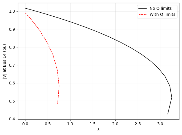
13.10. Reactive Power Limits

When PV.config.pv2pq is enabled, generators that hit their reactive power limits are converted from voltage control (PV) to fixed reactive power (PQ) at each corrector step. This reduces the maximum loadability because fewer generators maintain voltage support.

The following example compares the nose curve with and without Q-limit enforcement on the IEEE 14-bus system. The pv2pq setting must be passed at load time via config_option so that the internal limiter is initialized as enabled.

# Without Q limits (default)
ss_noq = andes.load(andes.get_case('ieee14/ieee14.json'))
ss_noq.PFlow.run()
ss_noq.CPF.run(load_scale=2.0)

# With Q limits — must be set at load time so the limiter is initialized enabled
ss_qlim = andes.load(andes.get_case('ieee14/ieee14.json'),
                     config_option=["PV.pv2pq=1"])
ss_qlim.PFlow.run()
ss_qlim.CPF.run(load_scale=2.0)

print(f"Max lambda without Q limits: {ss_noq.CPF.max_lam:.4f}")
print(f"Max lambda with Q limits:    {ss_qlim.CPF.max_lam:.4f}")

Max lambda without Q limits: 3.2580
Max lambda with Q limits:    0.7536

Working directory: "/home/docs/checkouts/readthedocs.org/user_builds/andes/checkouts/stable/docs/source/tutorials"
> Reloaded generated Python code of module "pycode".
Parsing input file "/home/docs/checkouts/readthedocs.org/user_builds/andes/envs/stable/lib/python3.11/site-packages/andes/cases/ieee14/ieee14.json"...
Input file parsed in 0.0020 seconds.
Connectivity check completed in 0.0001 seconds.
-> System connectivity check results:
  No islanded bus detected.
  System is interconnected.
  Each island has a slack bus correctly defined and enabled.
System internal structure set up in 0.0191 seconds.

-> Power flow calculation
           Numba: Off
   Sparse solver: KLU
 Solution method: NR method
Power flow initialized in 0.0032 seconds.
0: |F(x)| = 0.5605182134
1: |F(x)| = 0.006202200332
2: |F(x)| = 5.819382827e-06
3: |F(x)| = 6.957087684e-12
Converged in 4 iterations in 0.0020 seconds.
Report saved to "ieee14_out.txt" in 0.0006 seconds.

-> Continuation Power Flow
Parameterization: pseudo_arclength
       Step size: 0.1
   Adaptive step: On
         Stop at: NOSE
Nose detected at step 16, lambda=3.167739

-> CPF Report
       Converged: True
           Steps: 17
      Max lambda: 3.258046
     Termination: Nose point at lambda=3.258046
CPF completed in 17 steps in 0.0361 seconds. max lambda = 3.258046
Working directory: "/home/docs/checkouts/readthedocs.org/user_builds/andes/checkouts/stable/docs/source/tutorials"
> Reloaded generated Python code of module "pycode".
Generated code for <PV> is stale.
Numerical code generation (rapid incremental mode) started...
Generating code for 1 models on 2 processes.
Saved generated pycode to "/home/docs/.andes/pycode"
> Reloaded generated Python code of module "pycode".
Generated numerical code for 1 models in 0.1376 seconds.
Parsing input file "/home/docs/checkouts/readthedocs.org/user_builds/andes/envs/stable/lib/python3.11/site-packages/andes/cases/ieee14/ieee14.json"...
Input file parsed in 0.0021 seconds.
Connectivity check completed in 0.0001 seconds.
-> System connectivity check results:
  No islanded bus detected.
  System is interconnected.
  Each island has a slack bus correctly defined and enabled.
System internal structure set up in 0.0219 seconds.

-> Power flow calculation
           Numba: Off
   Sparse solver: KLU
 Solution method: NR method
Power flow initialized in 0.0033 seconds.
0: |F(x)| = 0.5605182134
1: |F(x)| = 0.006202200332
2: |F(x)| = 0.1543556844
3: |F(x)| = 0.05142223718
4: |F(x)| = 0.0005148845073
5: |F(x)| = 5.687884333e-08
Converged in 6 iterations in 0.0033 seconds.
Report saved to "ieee14_out.txt" in 0.0006 seconds.

-> Continuation Power Flow
Parameterization: pseudo_arclength
       Step size: 0.1
   Adaptive step: On
         Stop at: NOSE
Nose detected at step 7, lambda=0.722794

-> CPF Report
       Converged: True
           Steps: 8
      Max lambda: 0.753555
     Termination: Nose point at lambda=0.753555
CPF completed in 8 steps in 0.0169 seconds. max lambda = 0.753555

weak_noq = np.argmax(ss_noq.CPF.V[:, 0] - ss_noq.CPF.V[:, np.argmax(ss_noq.CPF.lam)])

fig, ax = plt.subplots()
ax.plot(ss_noq.CPF.lam, ss_noq.CPF.V[weak_noq, :], 'k-', linewidth=1.2, label='No Q limits')
ax.plot(ss_qlim.CPF.lam, ss_qlim.CPF.V[weak_noq, :], 'r--', linewidth=1.2, label='With Q limits')
ax.set_xlabel(r'$\lambda$')
ax.set_ylabel(f'|V| at Bus {ss_noq.Bus.idx.v[weak_noq]} (pu)')
ax.legend()
ax.grid(True, alpha=0.3)
fig.tight_layout()
plt.show()

13.11. Cleanup

!andes misc -C

"/home/docs/checkouts/readthedocs.org/user_builds/andes/checkouts/stable/docs/source/tutorials/ieee14_out.txt" removed.

13.12. Next Steps

• State Estimation: State estimation with WLS and custom measurements

• Eigenvalue Analysis: Small-signal stability assessment