8. Parameter Sweeps and Batch Processing#
Power system studies frequently require running many simulations with systematically varied parameters. You might want to understand how load levels affect voltage stability, how different fault locations impact system response, or how controller tuning parameters influence dynamic behavior. Rather than manually running each scenario one at a time, ANDES provides several approaches for batch processing that can dramatically reduce the time required for comprehensive studies.
This tutorial covers three approaches to batch simulation: file-based parallel processing for large studies, in-memory loops for smaller studies, and the pool option for intermediate cases where you want both parallelism and programmatic access to results.
Note
Prerequisites: This tutorial assumes familiarity with Python fundamentals including loops, dictionaries, and NumPy arrays. Complete First Simulation through Eigenvalue Analysis before proceeding.
8.1. Setup#
%matplotlib inline

import andes
import numpy as np
from matplotlib import pyplot as plt
import os
import shutil

andes.config_logger(stream_level=30)  # Reduce logging verbosity for batch runs
8.2. File-Based Batch Processing#
For large parametric studies involving hundreds or thousands of scenarios, the most efficient approach is to generate separate case files and then run them in parallel using the ANDES command-line interface. This approach leverages multi-core processors effectively and allows you to checkpoint progress by checking which output files exist.
8.2.1. Generating Case Files#
The workflow begins by loading a base case, modifying parameters programmatically, and saving each variation to a new file. In this example, we create three cases with load levels varying from 100% to 120% of the base value.
# Create output directory for the case files
os.makedirs('batch_cases', exist_ok=True)

# Load base case
kundur = andes.get_case('kundur/kundur_full.xlsx')
ss = andes.load(kundur)
# Get the base load value
p0_base = ss.PQ.get('p0', 'PQ_0')
print(f"Base load: {p0_base:.2f} MW")

# Create cases with load varying from 100% to 120% of base
N_CASES = 3
p0_values = np.linspace(p0_base, 1.2 * p0_base, N_CASES)

for value in p0_values:
    ss.PQ.set('p0', 'PQ_0', value, base='device')
    file_name = f'batch_cases/kundur_p_{value:.2f}.xlsx'
    andes.io.dump(ss, 'xlsx', file_name, overwrite=True)
    print(f"Created: {file_name}")
Base load: 11.59 MW
Created: batch_cases/kundur_p_11.59.xlsx
Created: batch_cases/kundur_p_12.75.xlsx
Created: batch_cases/kundur_p_13.91.xlsx
8.2.2. Running Cases in Parallel#
Once the case files are generated, you can run all of them in parallel using the andes run command with wildcards. ANDES automatically detects the number of CPU cores and distributes the workload across them.
# Run all cases with time-domain simulation
!andes run batch_cases/*.xlsx -r tds
    _           _         | Version 2.0.0
   /_\  _ _  __| |___ ___ | Python 3.11.12 on Linux, 03/12/2026 05:07:15 PM
  / _ \| ' \/ _` / -_|_-< |
 /_/ \_\_||_\__,_\___/__/ | This program comes with ABSOLUTELY NO WARRANTY.

Working directory: "/home/docs/checkouts/readthedocs.org/user_builds/andes/checkouts/stable/docs/source/tutorials"
> Loaded generated Python code in "/home/docs/.andes/pycode".
-> Processing 3 jobs on 2 CPUs.
  0%|                                                    | 0/100 [00:00<?, ?%/s]
 13%|#####2                                  | 13.0/100 [00:00<00:00, 128.87%/s]
 26%|##########6                              | 26.0/100 [00:00<00:00, 94.59%/s]
 37%|###############1                         | 37.0/100 [00:00<00:00, 93.07%/s]
 47%|###################2                     | 47.0/100 [00:00<00:00, 90.19%/s]
 57%|#######################3                 | 57.0/100 [00:00<00:00, 88.56%/s]
 66%|###########################              | 66.0/100 [00:00<00:00, 88.13%/s]
 74%|##############################3          | 74.0/100 [00:00<00:00, 87.10%/s]
 76%|###############################1         | 76.0/100 [00:00<00:00, 88.32%/s]
 83%|##################################       | 83.0/100 [00:00<00:00, 87.31%/s]
 86%|###################################2     | 86.0/100 [00:00<00:00, 89.90%/s]
 93%|######################################1  | 93.0/100 [00:01<00:00, 89.31%/s]
100%|########################################| 100.0/100 [00:01<00:00, 92.31%/s]
100%|########################################| 100.0/100 [00:01<00:00, 90.66%/s]
  0%|                                                    | 0/100 [00:00<?, ?%/s]
 13%|#####2                                  | 13.0/100 [00:00<00:00, 126.29%/s]
 26%|##########6                              | 26.0/100 [00:00<00:00, 95.48%/s]
 36%|##############7                          | 36.0/100 [00:00<00:00, 91.85%/s]
 46%|##################8                      | 46.0/100 [00:00<00:00, 90.42%/s]
 56%|######################9                  | 56.0/100 [00:00<00:00, 89.83%/s]
 66%|###########################              | 66.0/100 [00:00<00:00, 89.95%/s]
 76%|###############################1         | 76.0/100 [00:00<00:00, 91.46%/s]
 87%|###################################6     | 87.0/100 [00:00<00:00, 95.01%/s]
100%|########################################| 100.0/100 [00:01<00:00, 94.78%/s]
Log saved to "/tmp/andes-r0drvm2m/andes.log".
-> Multiprocessing finished in 3.5784 seconds.
If you need to limit CPU usage (for example, to leave resources for other tasks on a shared workstation), use the --ncpu flag to specify the maximum number of parallel processes.
# Limit to 2 parallel processes
!andes run batch_cases/*.xlsx -r tds --ncpu 2
    _           _         | Version 2.0.0
   /_\  _ _  __| |___ ___ | Python 3.11.12 on Linux, 03/12/2026 05:07:19 PM
  / _ \| ' \/ _` / -_|_-< |
 /_/ \_\_||_\__,_\___/__/ | This program comes with ABSOLUTELY NO WARRANTY.

Working directory: "/home/docs/checkouts/readthedocs.org/user_builds/andes/checkouts/stable/docs/source/tutorials"
> Loaded generated Python code in "/home/docs/.andes/pycode".
-> Processing 3 jobs on 2 CPUs.
  0%|                                                    | 0/100 [00:00<?, ?%/s]
  0%|                                                    | 0/100 [00:00<?, ?%/s]
 13%|#####2                                  | 13.0/100 [00:00<00:00, 127.61%/s]
 13%|#####2                                  | 13.0/100 [00:00<00:00, 125.89%/s]
 26%|##########6                              | 26.0/100 [00:00<00:00, 93.32%/s]
 36%|##############7                          | 36.0/100 [00:00<00:00, 90.22%/s]
 46%|##################8                      | 46.0/100 [00:00<00:00, 89.12%/s]
 46%|##################8                      | 46.0/100 [00:00<00:00, 87.10%/s]
 55%|######################5                  | 55.0/100 [00:00<00:00, 86.06%/s]
 64%|##########################2              | 64.0/100 [00:00<00:00, 85.58%/s]
 73%|#############################9           | 73.0/100 [00:00<00:00, 86.01%/s]
 82%|#################################6       | 82.0/100 [00:00<00:00, 86.58%/s]
 92%|#####################################7   | 92.0/100 [00:01<00:00, 88.11%/s]
100%|########################################| 100.0/100 [00:01<00:00, 90.02%/s]
100%|########################################| 100.0/100 [00:01<00:00, 89.33%/s]
  0%|                                                    | 0/100 [00:00<?, ?%/s]
 13%|#####2                                  | 13.0/100 [00:00<00:00, 126.47%/s]
 26%|##########6                              | 26.0/100 [00:00<00:00, 95.24%/s]
 36%|##############7                          | 36.0/100 [00:00<00:00, 91.56%/s]
 46%|##################8                      | 46.0/100 [00:00<00:00, 90.22%/s]
 56%|######################9                  | 56.0/100 [00:00<00:00, 89.64%/s]
 66%|###########################              | 66.0/100 [00:00<00:00, 89.74%/s]
 76%|###############################1         | 76.0/100 [00:00<00:00, 91.39%/s]
 87%|###################################6     | 87.0/100 [00:00<00:00, 94.51%/s]
 98%|########################################1| 98.0/100 [00:01<00:00, 97.00%/s]
100%|########################################| 100.0/100 [00:01<00:00, 94.55%/s]
Log saved to "/tmp/andes-oqy0sg97/andes.log".
-> Multiprocessing finished in 3.6100 seconds.
8.2.3. Returning System Objects for Post-Processing#
When you want to analyze results programmatically after batch execution, use pool=True in the Python API. This runs cases in parallel and returns a list of System objects that you can then analyze or plot.
# Run all cases and return System objects
systems = andes.run('batch_cases/*.xlsx', routine='tds', pool=True, verbose=30)

print(f"Completed {len(systems)} simulations")
print(f"Type of each result: {type(systems[0]).__name__}")
Completed 3 simulations
Type of each result: System
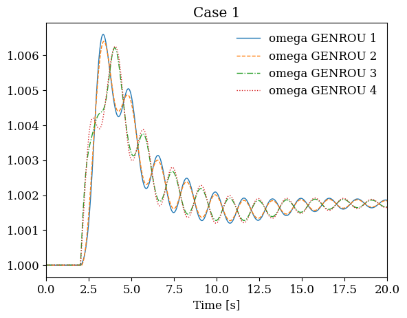
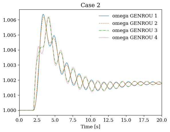
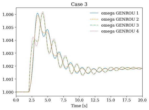
# Plot results from all cases side by side
fig, axes = plt.subplots(1, len(systems), figsize=(12, 4))

for i, sys in enumerate(systems):
    sys.TDS.plt.plot(sys.GENROU.omega, ax=axes[i],
                     title=f'Case {i+1}', latex=False, show=False)

plt.tight_layout()
plt.show()
8.3. In-Memory Parameter Sweeps#
For smaller studies where generating files would be unnecessary overhead, you can simply loop through parameter values in Python and accumulate results. This approach is particularly useful for quick exploratory analysis during model development or for sweeps involving only a few cases.
8.3.1. Power Flow Parameter Sweep#
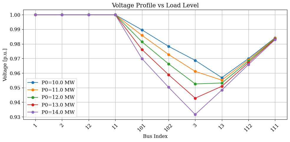
The following example sweeps load levels and records the resulting bus voltage profiles. Since power flow converges quickly, this type of sweep can complete in seconds even for many parameter values.
# Load system
ss = andes.run(kundur, no_output=True, default_config=True, verbose=30)

# View current load parameters
ss.PQ.as_df(vin=True)
| idx | u | name | bus | Vn | p0 | q0 | vmax | vmin | owner | |
|---|---|---|---|---|---|---|---|---|---|---|
| uid | ||||||||||
| 0 | PQ_0 | 1.0 | PQ_0 | 7 | 230.0 | 11.59 | -0.735 | 1.1 | 0.9 | 1 |
| 1 | PQ_1 | 1.0 | PQ_1 | 8 | 230.0 | 15.75 | -0.899 | 1.1 | 0.9 | 1 |
# Define parameter sweep range
n_samples = 5
pq0_values = np.linspace(10, 14, n_samples)  # MW range for PQ_0

# Storage for results: voltage at each bus for each parameter value
v_results = np.zeros((ss.Bus.n, n_samples))

# Run power flow for each load level
for i, p0 in enumerate(pq0_values):
    ss.PQ.set('p0', 'PQ_0', p0, base='device')
    ss.PFlow.run()
    v_results[:, i] = ss.dae.y[ss.Bus.v.a]

print(f"Completed {n_samples} power flow calculations")
Completed 5 power flow calculations
# Visualize how voltage profiles change with load level
plt.figure(figsize=(10, 5))
for i in range(n_samples):
    plt.plot(v_results[:, i], 'o-', label=f'P0={pq0_values[i]:.1f} MW')

plt.xlabel('Bus Index')
plt.ylabel('Voltage [p.u.]')
plt.title('Voltage Profile vs Load Level')
plt.legend()
plt.xticks(range(ss.Bus.n), ss.Bus.name.v, rotation=45)
plt.grid(True)
plt.tight_layout()
plt.show()
8.3.2. Batch Time-Domain Simulation#
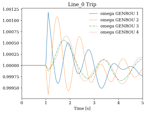
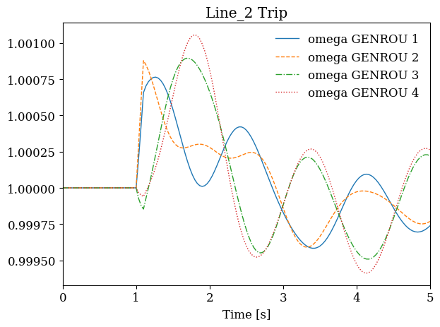
The same looping approach works for time-domain simulations, though each iteration takes longer. This example demonstrates running multiple contingency scenarios with different line trips. For each scenario, we create a fresh System object, add the appropriate disturbance, run the simulation, and store the result.
# Find available lines for contingency analysis
ss = andes.load(kundur, setup=False)
print(f"Available lines: {ss.Line.idx.v}")

# Select a subset for demonstration
lines_to_test = ss.Line.idx.v[:3]
Available lines: ['Line_0', 'Line_1', 'Line_2', 'Line_3', 'Line_4', 'Line_5', 'Line_6', 'Line_7', 'Line_8', 'Line_9', 'Line_10', 'Line_11', 'Line_12', 'Line_13', 'Line_14']
results = dict()

for line_idx in lines_to_test:
    # Load fresh system with setup=False to allow adding devices
    ss = andes.load(kundur, setup=False)

    # Add line trip at t=1.0s, restore at t=1.1s
    ss.add('Toggle', model='Line', dev=line_idx, t=1.0)
    ss.add('Toggle', model='Line', dev=line_idx, t=1.1)

    # Finalize system setup
    ss.setup()

    # Disable any existing Toggle from the test case
    ss.Toggle.set_status(1, 0)

    # Run simulation
    ss.PFlow.run()
    ss.TDS.config.tf = 5
    ss.TDS.config.no_tqdm = 1
    ss.TDS.run()

    results[line_idx] = ss
    print(f"Completed: {line_idx} trip")
Completed: Line_0 trip
Completed: Line_1 trip
Completed: Line_2 trip
# Compare generator response across contingencies
fig, axes = plt.subplots(1, len(results), figsize=(12, 4))

for ax, (line_idx, ss) in zip(axes, results.items()):
    ss.TDS.plt.plot(ss.GENROU.omega, ax=ax,
                    title=f'{line_idx} Trip', latex=False, show=False)

plt.tight_layout()
plt.show()

8.4. Choosing the Right Approach#
The following table summarizes when to use each batch processing technique:
Approach |
Best For |
Parallelism |
Memory Usage |
|---|---|---|---|
File-based CLI |
Large studies (>100 cases), production runs |
Multi-process |
Low (one case at a time) |
|
Medium studies, need results in memory |
Multi-process |
High (all results in memory) |
Python loop |
Small studies, rapid prototyping |
Single-thread |
Controlled (can discard results) |
For studies with more than about 10 cases, the file-based parallel approach is usually fastest because it fully utilizes all CPU cores. For smaller studies or when you are actively developing and testing, the simpler Python loop avoids the overhead of file I/O.
8.5. Cleanup#
shutil.rmtree('batch_cases', ignore_errors=True)
!andes misc -C
"/home/docs/checkouts/readthedocs.org/user_builds/andes/checkouts/stable/docs/source/tutorials/kundur_p_12.75_out.lst" removed.
"/home/docs/checkouts/readthedocs.org/user_builds/andes/checkouts/stable/docs/source/tutorials/kundur_full_out.txt" removed.
"/home/docs/checkouts/readthedocs.org/user_builds/andes/checkouts/stable/docs/source/tutorials/kundur_p_11.59_out.lst" removed.
"/home/docs/checkouts/readthedocs.org/user_builds/andes/checkouts/stable/docs/source/tutorials/kundur_p_12.75_out.txt" removed.
"/home/docs/checkouts/readthedocs.org/user_builds/andes/checkouts/stable/docs/source/tutorials/kundur_full_out.lst" removed.
"/home/docs/checkouts/readthedocs.org/user_builds/andes/checkouts/stable/docs/source/tutorials/kundur_p_12.75_out.npz" removed.
"/home/docs/checkouts/readthedocs.org/user_builds/andes/checkouts/stable/docs/source/tutorials/kundur_p_11.59_out.npz" removed.
"/home/docs/checkouts/readthedocs.org/user_builds/andes/checkouts/stable/docs/source/tutorials/kundur_p_13.91_out.lst" removed.
"/home/docs/checkouts/readthedocs.org/user_builds/andes/checkouts/stable/docs/source/tutorials/kundur_full_out.npz" removed.
"/home/docs/checkouts/readthedocs.org/user_builds/andes/checkouts/stable/docs/source/tutorials/kundur_p_13.91_out.npz" removed.
"/home/docs/checkouts/readthedocs.org/user_builds/andes/checkouts/stable/docs/source/tutorials/kundur_p_13.91_out.txt" removed.
"/home/docs/checkouts/readthedocs.org/user_builds/andes/checkouts/stable/docs/source/tutorials/kundur_p_11.59_out.txt" removed.
8.6. Next Steps#
Contingency Analysis - Systematic N-1 contingency screening
Dynamic Control and Setpoint Changes - Runtime parameter modifications
Frequency Response and Load Shedding - Frequency response analysis