11. Frequency Response and Load Shedding#
System frequency is a direct indicator of the real power balance between generation and load. When a generator trips unexpectedly, the remaining generators must pick up the lost generation through their turbine governors. If the generation shortfall is too large, frequency will decline until it stabilizes at a new (lower) value determined by the governor droop characteristics, or protective relays will disconnect loads to restore balance.
This tutorial demonstrates how to study frequency response in ANDES by simulating a generator trip and then implementing load shedding to restore frequency. These techniques are essential for understanding power system resilience and designing emergency control schemes.
Note
Prerequisites: Complete Time-Domain Simulation for disturbance simulation and Dynamic Control and Setpoint Changes for multi-stage simulation techniques.
11.1. Setup#
%matplotlib inline

import andes
import numpy as np

andes.config_logger(stream_level=20)
11.2. Simulating a Generator Trip#
We use the IEEE 14-bus system, which includes generators with turbine governors and exciters. The Toggle device can disconnect any component, including generators. We will trip one of the generators and observe the frequency response of the remaining machines.
First, load the system with setup=False so we can add the Toggle before finalizing the system structure.
ieee14_raw = andes.get_case("ieee14/ieee14.raw")
ieee14_dyr = andes.get_case("ieee14/ieee14.dyr")

ss = andes.load(ieee14_raw, addfile=ieee14_dyr, setup=False)
Working directory: "/home/docs/checkouts/readthedocs.org/user_builds/andes/checkouts/stable/docs/source/tutorials"
> Loaded generated Python code in "/home/docs/.andes/pycode".
Parsing input file "/home/docs/checkouts/readthedocs.org/user_builds/andes/envs/stable/lib/python3.11/site-packages/andes/cases/ieee14/ieee14.raw"...
  IEEE 14 BUS TEST CASE
  03/06/14 CONTO           100.0  1962 W
Input file parsed in 0.0596 seconds.
Parsing additional file "/home/docs/checkouts/readthedocs.org/user_builds/andes/envs/stable/lib/python3.11/site-packages/andes/cases/ieee14/ieee14.dyr"...
Addfile parsed in 0.2950 seconds.
# Add a Toggle to trip GENROU_2 at t=1 second
ss.add("Toggle", model='SynGen', dev="GENROU_2", t=1.0)

# Complete system setup
ss.setup()
IEEEST <IEEEST_1> added BusFreq <BusFreq_1> linked to bus <3.0>
ST2CUT <ST2CUT_2> added BusFreq <BusFreq_2> linked to bus <1.0>
ST2CUT <ST2CUT_3> added BusFreq <BusFreq_3> linked to bus <2.0>
Connectivity check completed in 0.0001 seconds.
-> System connectivity check results:
  No islanded bus detected.
  System is interconnected.
  Each island has a slack bus correctly defined and enabled.
System internal structure set up in 0.0222 seconds.
True
The IEEE 14-bus test case includes pre-defined Toggle devices for line switching. We disable them to study the generator trip in isolation.
# View all Toggle devices
ss.Toggle.as_df()
| idx | u | name | model | dev | t | |
|---|---|---|---|---|---|---|
| uid | ||||||
| 0 | Toggle_1 | 1.0 | Toggle_1 | Line | Line_1 | 1.0 |
| 1 | Toggle_2 | 1.0 | Toggle_2 | Line | Line_1 | 1.1 |
| 2 | Toggle_3 | 1.0 | Toggle_3 | SynGen | GENROU_2 | 1.0 |
# Disable the line switching Toggles (indices 0 and 1)
ss.Toggle.u.v[[0, 1]] = 0
For this study, we configure the PQ loads to use constant power (rather than constant impedance) behavior during the simulation. This makes the frequency response more pronounced because the loads do not naturally decrease as voltage drops.
# Configure PQ loads for constant power behavior
ss.PQ.config.p2p = 1  # Active power: 100% constant P
ss.PQ.config.q2q = 1  # Reactive power: 100% constant Q
ss.PQ.config.p2z = 0  # No constant impedance component
ss.PQ.config.q2z = 0

# Disable under-voltage PQ-to-Z conversion
ss.PQ.pq2z = 0
# Run power flow and time-domain simulation
ss.PFlow.run()

ss.TDS.config.tf = 20
ss.TDS.config.criteria = 0  # Disable angle separation criterion (for this study)
ss.TDS.run()
-> Power flow calculation
           Numba: Off
   Sparse solver: KLU
 Solution method: NR method
Power flow initialized in 0.0039 seconds.
0: |F(x)| = 0.5605182134
1: |F(x)| = 0.006202200332
2: |F(x)| = 5.819382827e-06
3: |F(x)| = 6.957087684e-12
Converged in 4 iterations in 0.0023 seconds.
Report saved to "ieee14_out.txt" in 0.0007 seconds.
DAE compaction: removed 6 algebraic variable slots (m: 246 -> 240)
Initialization for dynamics completed in 0.0261 seconds.
Initialization was successful.
<Toggle Toggle_3>: SynGen.GENROU_2 status changed to 0 at t=1.0 sec.
Simulation to t=20.00 sec completed in 2.4786 seconds.
Outputs to "ieee14_out.lst" and "ieee14_out.npz".
Outputs written in 0.0423 seconds.
True
Now let us plot the frequency of the remaining online generators. We multiply by 60 to convert from per-unit to Hz (for a 60 Hz system). Generator GENROU_2 (index 1) was tripped, so we plot only the remaining machines.
ss.TDS.load_plotter()

fig, ax = ss.TDS.plt.plot(
    ss.GENROU.omega,
    a=(0, 2, 3, 4),  # Exclude tripped generator (index 1)
    ytimes=60,
    ylabel='Frequency [Hz]'
)
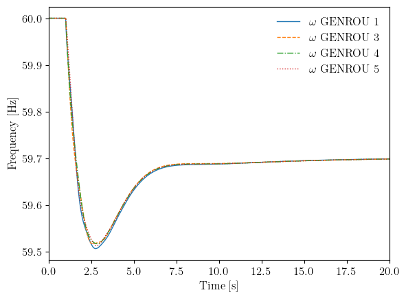
The plot shows the classic frequency response to a generation loss: an immediate frequency decline as the generators decelerate, followed by governor action that gradually arrests the decline. The frequency settles at a new steady-state value below nominal (60 Hz) because the governors have droop characteristics rather than isochronous control.
To restore frequency to nominal, either more generation must be added or load must be shed.
11.3. Determining the Generation Shortfall#
Before implementing load shedding, we need to know how much generation was lost. This information comes from the power flow solution for the tripped generator.
# View PV generator data
ss.PV.as_df()[['idx', 'bus', 'p0', 'q0']]
| idx | bus | p0 | q0 | |
|---|---|---|---|---|
| uid | ||||
| 0 | 2 | 2 | 0.40 | 0.15 |
| 1 | 3 | 3 | 0.40 | 0.15 |
| 2 | 4 | 6 | 0.30 | 0.10 |
| 3 | 5 | 8 | 0.35 | 0.10 |
GENROU_2 corresponds to the first PV generator (GENROU_1 corresponds to the Slack bus). The lost active power is 0.40 pu on the 100 MVA system base, which equals 40 MW.
11.4. Implementing Load Shedding#
We now reload the system and implement a two-stage simulation: first let the frequency decline after the generator trip, then shed 0.4 pu of load at t=2 seconds to compensate for the lost generation.
Load shedding is implemented by reducing the Ppf (power flow active power) parameter of selected PQ loads. This is the parameter that the PQ model uses during time-domain simulation when configured for constant power behavior.
# Reload the system
ss = andes.load(ieee14_raw, addfile=ieee14_dyr, setup=False)

ss.add("Toggle", model='SynGen', dev="GENROU_2", t=1.0)
ss.setup()
ss.Toggle.u.v[[0, 1]] = 0

ss.PQ.config.p2p = 1
ss.PQ.config.q2q = 1
ss.PQ.config.p2z = 0
ss.PQ.config.q2z = 0
ss.PQ.pq2z = 0

ss.PFlow.run()
Working directory: "/home/docs/checkouts/readthedocs.org/user_builds/andes/checkouts/stable/docs/source/tutorials"
> Reloaded generated Python code of module "pycode".
Parsing input file "/home/docs/checkouts/readthedocs.org/user_builds/andes/envs/stable/lib/python3.11/site-packages/andes/cases/ieee14/ieee14.raw"...
  IEEE 14 BUS TEST CASE
  03/06/14 CONTO           100.0  1962 W
Input file parsed in 0.0057 seconds.
Parsing additional file "/home/docs/checkouts/readthedocs.org/user_builds/andes/envs/stable/lib/python3.11/site-packages/andes/cases/ieee14/ieee14.dyr"...
Addfile parsed in 0.0824 seconds.
IEEEST <IEEEST_1> added BusFreq <BusFreq_1> linked to bus <3.0>
ST2CUT <ST2CUT_2> added BusFreq <BusFreq_2> linked to bus <1.0>
ST2CUT <ST2CUT_3> added BusFreq <BusFreq_3> linked to bus <2.0>
Connectivity check completed in 0.0001 seconds.
-> System connectivity check results:
  No islanded bus detected.
  System is interconnected.
  Each island has a slack bus correctly defined and enabled.
System internal structure set up in 0.0198 seconds.

-> Power flow calculation
           Numba: Off
   Sparse solver: KLU
 Solution method: NR method
Power flow initialized in 0.0033 seconds.
0: |F(x)| = 0.5605182134
1: |F(x)| = 0.006202200332
2: |F(x)| = 5.819382827e-06
3: |F(x)| = 6.957087684e-12
Converged in 4 iterations in 0.0021 seconds.
Report saved to "ieee14_out.txt" in 0.0006 seconds.
True
# Run simulation to t=2 seconds (generator trips at t=1s)
ss.TDS.config.tf = 2.0
ss.TDS.config.criteria = 0
ss.TDS.run()
DAE compaction: removed 6 algebraic variable slots (m: 246 -> 240)
Initialization for dynamics completed in 0.0258 seconds.
Initialization was successful.
<Toggle Toggle_3>: SynGen.GENROU_2 status changed to 0 at t=1.0 sec.
Simulation to t=2.00 sec completed in 0.3182 seconds.
Outputs to "ieee14_out.lst" and "ieee14_out.npz".
Outputs written in 0.0035 seconds.
True
Now we shed load by reducing the active power of loads on selected buses. We distribute the 0.4 pu load reduction equally among six buses.
# Select buses for load shedding
shed_buses = [2, 3, 4, 5, 6, 9]

# Find the PQ device indices on these buses
pq_shed_idx = ss.PQ.find_idx(keys='bus', values=shed_buses)
print(f"PQ devices to shed: {pq_shed_idx}")
PQ devices to shed: ['PQ_1', 'PQ_2', 'PQ_3', 'PQ_4', 'PQ_5', 'PQ_6']
# Get current active power values
pq_p = ss.PQ.get(src='Ppf', idx=pq_shed_idx, attr='v')
print(f"Current load values: {pq_p}")

# Calculate new values after shedding (distribute 0.4 pu equally)
pq_p_new = pq_p - 0.4 / len(shed_buses)
print(f"New load values: {pq_p_new}")

# Apply the load shedding
ss.PQ.set('Ppf', pq_shed_idx, pq_p_new)
Current load values: [0.217 0.5   0.478 0.076 0.15  0.295]
New load values: [0.15033333 0.43333333 0.41133333 0.00933333 0.08333333 0.22833333]
True
# Continue simulation to 10 seconds
ss.TDS.config.tf = 10
ss.TDS.run()
Simulation to t=10.00 sec completed in 1.0669 seconds.
Outputs to "ieee14_out.lst" and "ieee14_out.npz".
Outputs written in 0.0205 seconds.
True
fig, ax = ss.TDS.plt.plot(
    ss.GENROU.omega,
    a=(0, 2, 3, 4),
    ytimes=60,
    ylabel='Frequency [Hz]'
)
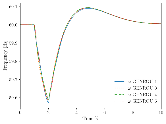
The plot now shows two distinct phases:
t=1-2s: Frequency declines after the generator trip as the remaining generators decelerate
t=2-10s: After load shedding at t=2s, frequency recovers back toward 60 Hz
The frequency returns to approximately 60 Hz because we shed exactly the amount of load equal to the lost generation. In practice, under-frequency load shedding (UFLS) schemes are designed with multiple stages that trigger at progressively lower frequencies.
11.5. Key Concepts#
Concept |
Description |
|---|---|
Governor droop |
Governors respond to frequency deviation proportionally, leading to a new steady-state frequency below nominal |
Load shedding |
Disconnecting loads to restore generation-load balance |
UFLS |
Under-Frequency Load Shedding - automated schemes that trip loads at preset frequency thresholds |
Rate of Change of Frequency (RoCoF) |
How quickly frequency changes after a disturbance, related to system inertia |
11.6. Cleanup#
!andes misc -C
"/home/docs/checkouts/readthedocs.org/user_builds/andes/checkouts/stable/docs/source/tutorials/ieee14_out.npz" removed.
"/home/docs/checkouts/readthedocs.org/user_builds/andes/checkouts/stable/docs/source/tutorials/ieee14_out.txt" removed.
"/home/docs/checkouts/readthedocs.org/user_builds/andes/checkouts/stable/docs/source/tutorials/ieee14_out.lst" removed.
11.7. Next Steps#
Eigenvalue Analysis - Small-signal stability analysis
Contingency Analysis - Systematic contingency screening
Dynamic Control and Setpoint Changes - Runtime parameter modifications