9. Contingency Analysis

Contingency analysis is a critical component of power system planning and operations. It evaluates how the system responds to various disturbances, typically single component outages known as "N-1" contingencies. By systematically simulating line trips, generator outages, and bus faults, you can identify weak points in the system that might lead to voltage collapse or loss of synchronism.

This tutorial demonstrates how to perform systematic contingency screening using ANDES. We cover N-1 line contingencies, generator trips, fault-and-clear analysis, and methods for assessing stability from simulation results.

Note

Prerequisites: This tutorial uses Python functions and pandas DataFrames. Complete Time-Domain Simulation for disturbance basics and Parameter Sweeps and Batch Processing for batch simulation patterns before proceeding.

9.1. Setup

%matplotlib inline

import andes
import numpy as np
import pandas as pd
from matplotlib import pyplot as plt

andes.config_logger(stream_level=30)  # Reduce verbosity for batch runs

case_file = andes.get_case('kundur/kundur_full.xlsx')

9.2. N-1 Line Contingency Screening

The most common contingency analysis involves testing the loss of each transmission line individually. For each line, we load a fresh system, add a Toggle device to trip the line at a specified time, run the simulation, and then assess whether the system remained stable.

First, let us identify all available lines in the test case.

# Load system to inspect lines
ss = andes.load(case_file, setup=False)
all_lines = list(ss.Line.idx.v)
print(f"Lines in the system: {all_lines}")

Lines in the system: ['Line_0', 'Line_1', 'Line_2', 'Line_3', 'Line_4', 'Line_5', 'Line_6', 'Line_7', 'Line_8', 'Line_9', 'Line_10', 'Line_11', 'Line_12', 'Line_13', 'Line_14']

Now we loop through each line and simulate its outage. For demonstration purposes, we test only the first three lines to keep execution time reasonable. In a real study, you would test all lines.

# Select subset for demonstration
lines_to_test = all_lines[:3]

results = {}
for line_idx in lines_to_test:
    # Load fresh system with setup=False to allow adding devices
    ss = andes.load(case_file, setup=False)

    # Add line trip at t=1.0s
    ss.add('Toggle', model='Line', dev=line_idx, t=1.0)

    ss.setup()

    # Disable existing Toggle in base case
    ss.Toggle.set_status(1, 0)

    ss.PFlow.run()
    ss.TDS.config.tf = 5
    ss.TDS.config.no_tqdm = 1
    ss.TDS.run()

    # Record max generator speed deviation as a stability metric
    omega = ss.dae.ts.x[:, ss.GENROU.omega.a]
    omega_max = omega.max()
    omega_min = omega.min()

    results[line_idx] = {
        'omega_max': omega_max,
        'omega_min': omega_min,
        'exit_code': ss.exit_code,
        'system': ss
    }

    print(f"{line_idx}: omega_max={omega_max:.4f}, omega_min={omega_min:.4f}")

Line_0: omega_max=1.0050, omega_min=0.9988
Line_1: omega_max=1.0050, omega_min=0.9988
Line_2: omega_max=1.0085, omega_min=0.9998

9.3. Stability Assessment

After running simulations, we need to determine which contingencies resulted in stable operation and which caused problems. Common stability criteria include:

• Generator speeds should remain within acceptable bounds (typically 0.95-1.05 pu)

• Bus voltages should stay above minimum thresholds (typically 0.8 pu)

• The simulation should complete without numerical failures

The following function encapsulates these checks.

Tip

The screening loop above and the function below use direct DAE array indexing (ss.dae.ts.x[:, addr]) for speed in batch loops. For interactive analysis or single simulations, ss.TDS.get_timeseries(ss.GENROU.omega) returns the same data as a pandas DataFrame — see Time-Domain Simulation for details.

def assess_stability(ss):
    """Return stability assessment for a completed simulation."""

    if ss.exit_code != 0:
        return {'stable': False, 'reason': 'simulation_failed'}

    omega = ss.dae.ts.x[:, ss.GENROU.omega.a]
    v = ss.dae.ts.y[:, ss.Bus.v.a]

    omega_max = omega.max()
    omega_min = omega.min()
    v_min = v.min()

    stable = (omega_max < 1.05 and omega_min > 0.95 and v_min > 0.8)

    return {
        'stable': stable,
        'omega_max': omega_max,
        'omega_min': omega_min,
        'v_min': v_min
    }

# Generate contingency report
records = []
for cont_id, data in results.items():
    metrics = assess_stability(data['system'])
    records.append({
        'contingency': cont_id,
        **metrics
    })

df = pd.DataFrame(records)
df

	contingency	stable	omega_max	omega_min	v_min
0	Line_0	True	1.005020	0.998823	0.880968
1	Line_1	True	1.005018	0.998824	0.881003
2	Line_2	True	1.008547	0.999849	0.830137

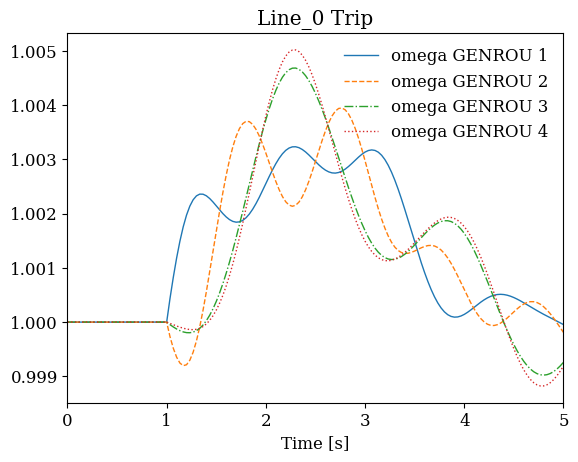
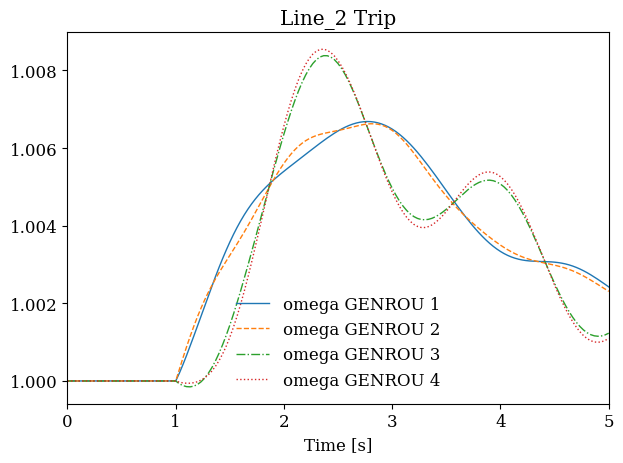
9.4. Visualizing Contingency Results

Plotting the generator response for each contingency provides insight into the system dynamics and helps identify which modes are excited by different disturbances.

fig, axes = plt.subplots(1, len(results), figsize=(12, 4))

for ax, (line_idx, data) in zip(axes, results.items()):
    ss = data['system']
    ss.TDS.plt.plot(ss.GENROU.omega, ax=ax,
                    title=f'{line_idx} Trip', latex=False, show=False)

plt.tight_layout()
plt.show()

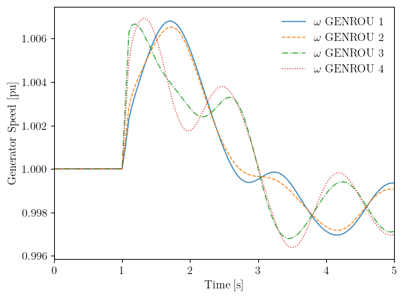
9.5. Fault-and-Clear Analysis

Three-phase faults followed by fault clearing represent more severe disturbances than simple line trips. The severity depends on both the fault location (which bus) and the fault duration (clearing time). Faults near generators or at critical buses can cause rapid acceleration of nearby machines.

In ANDES, faults are modeled using the Fault device with tf (fault time) and tc (clearing time) parameters.

# Get bus indices for fault analysis
ss = andes.load(case_file, setup=False)
print(f"Available buses: {ss.Bus.idx.v}")

Available buses: [1, 2, 3, 4, 5, 6, 7, 8, 9, 10]

# Test 100ms fault at bus 3
ss = andes.load(case_file, setup=False)

# Add fault at t=1.0s, clear at t=1.1s (100ms duration)
ss.add('Fault', bus=3, tf=1.0, tc=1.1)

ss.setup()

# Disable existing Toggle in base case
ss.Toggle.set_status(1, 0)

ss.PFlow.run()
ss.TDS.config.tf = 5
ss.TDS.run()

True

# Plot response to fault
fig, ax = ss.TDS.plt.plot(ss.GENROU.omega, ylabel='Generator Speed [pu]')

9.6. Critical Clearing Time

Critical Clearing Time (CCT) is the maximum fault duration for which the system remains stable. It is a key metric for protection system coordination. Finding CCT involves a binary search: if the system is stable at a given clearing time, we try a longer fault; if unstable, we try a shorter fault.

The following function implements this binary search.

def find_cct(case_file, bus_idx, t_fault=1.0,
             tc_min=0.05, tc_max=0.5, tol=0.02):
    """Binary search for critical clearing time.

    Parameters
    ----------
    case_file : str
        Path to the case file
    bus_idx : int or str
        Bus index for the fault
    t_fault : float
        Fault initiation time
    tc_min : float
        Minimum clearing time to test
    tc_max : float
        Maximum clearing time to test
    tol : float
        Tolerance for binary search (seconds)

    Returns
    -------
    float
        Estimated critical clearing time
    """
    iterations = 0
    max_iterations = 20  # Safety limit

    while (tc_max - tc_min) > tol and iterations < max_iterations:
        tc_mid = (tc_min + tc_max) / 2

        ss = andes.load(case_file, setup=False)
        ss.add('Fault', bus=bus_idx, tf=t_fault, tc=t_fault + tc_mid)
        ss.setup()

        # Disable existing Toggle
        ss.Toggle.set_status(1, 0)

        ss.PFlow.run()
        ss.TDS.config.tf = 5
        ss.TDS.config.no_tqdm = 1
        ss.TDS.run()

        metrics = assess_stability(ss)

        if metrics['stable']:
            tc_min = tc_mid  # Stable, try longer fault
        else:
            tc_max = tc_mid  # Unstable, try shorter fault

        iterations += 1

    return tc_min

# Find CCT for bus 3
cct = find_cct(case_file, bus_idx=3)
print(f"Critical Clearing Time for Bus 3: {cct*1000:.0f} ms")

Critical Clearing Time for Bus 3: 50 ms

9.7. Stability Metrics Summary

The following table summarizes common metrics used in contingency screening:

Metric	Description	Typical Threshold
omega_max	Maximum generator speed	< 1.05 pu
omega_min	Minimum generator speed	> 0.95 pu
v_min	Minimum bus voltage	> 0.8 pu
exit_code	Simulation completion	== 0
CCT	Critical clearing time	Depends on protection

These thresholds should be adjusted based on the specific system and operating standards applicable to your study.

9.8. Cleanup

!andes misc -C

"/home/docs/checkouts/readthedocs.org/user_builds/andes/checkouts/stable/docs/source/tutorials/kundur_full_out.txt" removed.
"/home/docs/checkouts/readthedocs.org/user_builds/andes/checkouts/stable/docs/source/tutorials/kundur_full_out.lst" removed.
"/home/docs/checkouts/readthedocs.org/user_builds/andes/checkouts/stable/docs/source/tutorials/kundur_full_out.npz" removed.

9.9. Next Steps

• Dynamic Control and Setpoint Changes - Runtime parameter modifications

• Frequency Response and Load Shedding - Frequency response analysis

• Parameter Sweeps and Batch Processing - Batch simulation techniques