6. Plotting Results

Effective visualization is essential for understanding power system dynamics. After running a time-domain simulation, you typically want to examine how variables like generator speeds, bus voltages, and power flows change over time. ANDES provides a built-in plotting interface through ss.TDS.plt that makes it easy to create publication-quality figures with minimal code.

This tutorial covers the plotting capabilities available in ANDES, from basic variable plotting to customization options and exporting results. By the end, you will be able to create informative plots that clearly communicate simulation results.

6.1. Setup and Run Simulation

Before we can plot results, we need simulation data. Let us run a time-domain simulation on the Kundur two-area system, which contains a line trip disturbance that triggers interesting oscillatory dynamics.

%matplotlib inline

import andes

andes.config_logger(stream_level=20)

# Load system and run power flow
ss = andes.load(andes.get_case('kundur/kundur_full.xlsx'))
ss.PFlow.run()

# Run time-domain simulation
ss.TDS.config.tf = 10
ss.TDS.run()

Working directory: "/home/docs/checkouts/readthedocs.org/user_builds/andes/checkouts/stable/docs/source/tutorials"
> Loaded generated Python code in "/home/docs/.andes/pycode".
Parsing input file "/home/docs/checkouts/readthedocs.org/user_builds/andes/envs/stable/lib/python3.11/site-packages/andes/cases/kundur/kundur_full.xlsx"...
Input file parsed in 0.0315 seconds.
Connectivity check completed in 0.0001 seconds.
-> System connectivity check results:
  No islanded bus detected.
  System is interconnected.
  Each island has a slack bus correctly defined and enabled.
System internal structure set up in 0.0205 seconds.

-> Power flow calculation
           Numba: Off
   Sparse solver: KLU
 Solution method: NR method
Power flow initialized in 0.0031 seconds.
0: |F(x)| = 14.9282832
1: |F(x)| = 3.608627841
2: |F(x)| = 0.1701107882
3: |F(x)| = 0.002038626956
4: |F(x)| = 3.745103977e-07
Converged in 5 iterations in 0.0025 seconds.
Report saved to "kundur_full_out.txt" in 0.0008 seconds.
DAE compaction: removed 5 algebraic variable slots (m: 149 -> 144)
Initialization for dynamics completed in 0.0152 seconds.
Initialization was successful.
<Toggle 1>: Line.Line_8 status changed to 0 at t=2.0 sec.
Simulation to t=10.00 sec completed in 0.5439 seconds.
Outputs to "kundur_full_out.lst" and "kundur_full_out.npz".
Outputs written in 0.0142 seconds.

True

6.2. The Plotter Object

When running ANDES interactively (in Jupyter Notebook or IPython), a plotter object is automatically created at ss.TDS.plt after time-domain simulation completes. This object provides methods for plotting variables, finding variable indices, and exporting data.

You can verify that the plotter was created successfully by checking its type.

ss.TDS.plt

<andes.plot.TDSData at 0x7d3c2fc56b90>

If ss.TDS.plt is None (which can happen if the interactive environment detection fails), you can manually create it by calling ss.TDS.load_plotter(). This step is normally not needed but is useful to know about for troubleshooting.

ss.TDS.load_plotter()

6.3. Plotting by Variable

The most straightforward way to plot simulation results is by passing a variable object directly to the plot() method. This approach is intuitive because you reference the exact quantity you want to visualize without needing to look up numerical indices.

For example, to plot all generator rotor speeds (the omega variable of the GENROU model), simply pass ss.GENROU.omega to the plotter.

fig, ax = ss.TDS.plt.plot(ss.GENROU.omega)

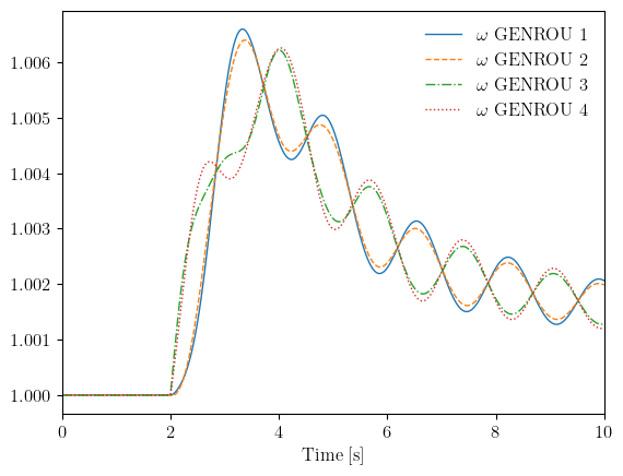
The plot shows the characteristic inter-area oscillations of the Kundur two-area system. After the line trips at t=2s, generators in the same area swing together while generators in different areas swing against each other. This inter-area mode is a key concern in power system stability analysis.

The plot() method returns both a figure object and an axis object, which you can use for further customization with matplotlib.

6.3.1. Plotting a Subset of Variables

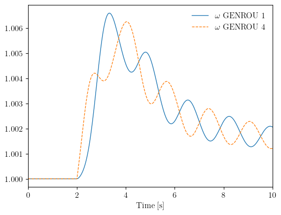
When a model has many instances, you may only want to plot a subset rather than all of them. The a argument accepts a tuple of zero-indexed positions indicating which variables to include.

For example, to plot only the first and fourth generators (positions 0 and 3), use:

fig, ax = ss.TDS.plt.plot(ss.GENROU.omega, a=(0, 3))

You can also plot bus voltage magnitudes. The bus voltage variable v is accessed through ss.Bus.v (note that this is an algebraic variable rather than a state variable like generator speed).

fig, ax = ss.TDS.plt.plot(ss.Bus.v)

6.4. Index-Based Plotting

For more advanced use cases or when working with the command-line plotting tool, you may need to plot by variable index rather than by variable object. ANDES assigns each variable a unique index that is recorded in the output .lst file.

The find() method helps you discover these indices. It searches variable names using patterns (with regular expression support) and returns both the indices and the matching variable names.

# Find all variables containing 'omega'
ss.TDS.plt.find('omega')

([5, 6, 7, 8],
 ['omega GENROU 1', 'omega GENROU 2', 'omega GENROU 3', 'omega GENROU 4'])

Once you know the indices, you can pass them as a tuple or list to plot(). This produces the same result as plotting by variable but uses the numerical indices instead.

# Plot using indices directly
fig, ax = ss.TDS.plt.plot((5, 6, 7, 8))

The index-based approach is particularly useful when using the andes plot command from the terminal:

andes plot kundur_full_out.lst 0 5 6 7 8

Here, index 0 represents time, and indices 5-8 represent the generator speeds.

6.5. Customizing Plots

The plot() method accepts numerous arguments for customizing the appearance of your figures. These options let you create publication-ready plots without needing to write additional matplotlib code.

6.5.1. Labels and Legends

fig, ax = ss.TDS.plt.plot(
    ss.GENROU.omega,
    ylabel='Generator Speed [pu]',
    yheader=['Gen 1', 'Gen 2', 'Gen 3', 'Gen 4']
)

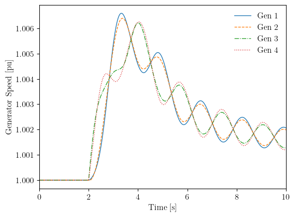
The ylabel argument sets the y-axis label, while yheader provides custom legend entries. When using yheader, ensure the number of entries matches the number of variables being plotted.

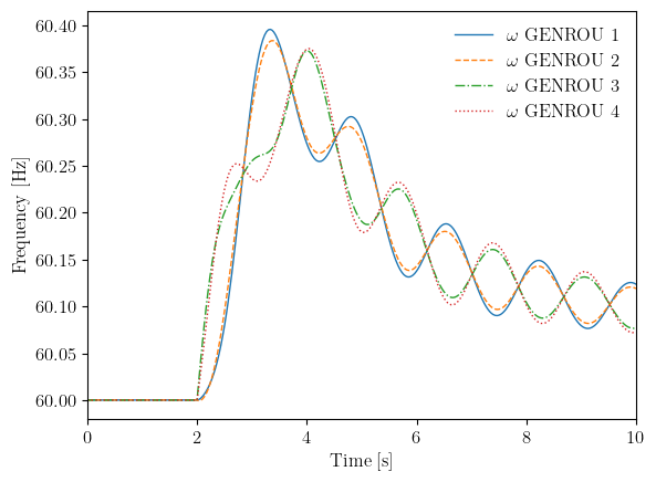
6.5.2. Scaling Values

Power system variables are often stored in per-unit but may be more intuitive when displayed in other units. The ycalc argument accepts a callable that transforms the y-values before plotting.

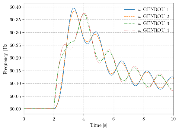
For example, to convert generator speed from per-unit to Hz (for a 60 Hz system where 1.0 pu = 60 Hz):

fig, ax = ss.TDS.plt.plot(
    ss.GENROU.omega,
    ycalc=lambda x: 60 * x,
    ylabel='Frequency [Hz]'
)

6.5.3. Grid and Greyscale

For technical publications or presentations, you may want to add a grid for easier reading or use greyscale for black-and-white printing.

fig, ax = ss.TDS.plt.plot(
    ss.GENROU.omega,
    ycalc=lambda x: 60 * x,
    ylabel='Frequency [Hz]',
    grid=True,
    greyscale=True
)

6.5.4. Adding Curves to an Existing Figure

When comparing results from different scenarios or showing related variables on the same plot, you can add new curves to an existing figure. Pass the fig and ax objects from a previous plot to overlay new data.

# First plot: generators 1 and 4
fig, ax = ss.TDS.plt.plot(ss.GENROU.omega, a=(0, 3))

# Add generator 2 with a different line style
fig, ax = ss.TDS.plt.plot(
    ss.GENROU.omega,
    a=(1,),
    fig=fig,
    ax=ax,
    linestyles=['-.']
)

<Figure size 640x480 with 0 Axes>

6.6. Interactive Plots with Plotly

For exploratory analysis in Jupyter notebooks, ANDES supports an interactive Plotly backend. Plotly figures support zooming, panning, and hover tooltips that show exact values — all without any extra code.

To use it, pass backend='plotly' to the plot() method. The API is otherwise identical to the default matplotlib backend.

fig = ss.TDS.plt.plot(ss.GENROU.omega, backend='plotly')

All customization arguments (ylabel, grid, ytimes, hline, vline, axis limits, etc.) work the same way as with matplotlib. LaTeX legend labels are automatically replaced with plain text since Plotly does not render LaTeX in legends.

fig = ss.TDS.plt.plot(
    ss.GENROU.omega,
    ytimes=60,
    ylabel='Frequency [Hz]',
    title='Generator Frequencies',
    hline=60.0,
    grid=True,
    backend='plotly',
)

6.7. Saving Figures

Figures can be saved directly from the plot() method using the savefig argument. When set to True, the figure is saved with an automatically generated filename. You can also pass a string to specify the exact filename.

fig, ax = ss.TDS.plt.plot(
    ss.GENROU.omega,
    ylabel='Generator Speed [pu]',
    savefig='generator_speeds.png'
)

Figure saved to "generator_speeds.png".

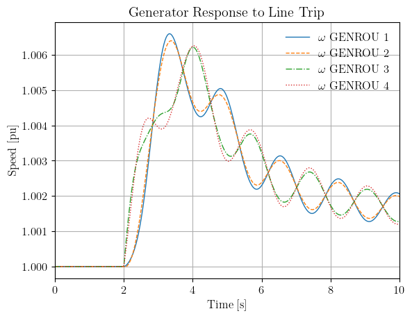
For more control over the output format and resolution, you can save the figure using matplotlib directly. This is useful when you need vector formats like PDF for publications.

fig, ax = ss.TDS.plt.plot(ss.GENROU.omega, show=False)
ax.set_title('Generator Response to Line Trip')
ax.set_ylabel('Speed [pu]')
ax.grid(True)
fig.savefig('generator_response.pdf', dpi=300, bbox_inches='tight')

6.8. Exporting to CSV

While plots are useful for visualization, you often need the raw numerical data for further analysis in spreadsheets or other tools. The export_csv() method exports all simulation results to a CSV file that can be opened in Excel or read by other programs.

ss.TDS.plt.export_csv('simulation_results.csv')

CSV data saved to "simulation_results.csv".

'simulation_results.csv'

For more selective export, the get_timeseries() method returns a pandas DataFrame for any variable, ready for further analysis. For advanced use, the underlying arrays are accessible through ss.dae.ts (see Time-Domain Simulation).

# Get time series as DataFrames
omega_df = ss.TDS.get_timeseries(ss.GENROU.omega)
voltage_df = ss.TDS.get_timeseries(ss.Bus.v)

# Combine selected columns
import pandas as pd
df = pd.DataFrame({
    'Gen1_omega': omega_df.iloc[:, 0],
    'Gen2_omega': omega_df.iloc[:, 1],
    'Bus1_v': voltage_df.iloc[:, 0],
})
df.head()

	Gen1_omega	Gen2_omega	Bus1_v
0.000000	1.0	1.0	1.0
0.033333	1.0	1.0	1.0
0.066667	1.0	1.0	1.0
0.100000	1.0	1.0	1.0
0.133333	1.0	1.0	1.0

df.to_csv('selected_results.csv', index=False)

6.9. Plot Method Reference

The plot() method supports many additional arguments for fine-grained control. Here is a summary of the most commonly used options:

Argument	Description
a	Tuple of indices to select subset of variables
ylabel	Y-axis label
yheader	List of legend entries
ycalc	Callable to transform y-values
grid	Show grid lines (True/False)
greyscale	Use greyscale colors (True/False)
savefig	Save figure (True or filename)
dpi	Resolution for saved figure
left, right	X-axis limits
ymin, ymax	Y-axis limits
fig, ax	Existing figure/axis to plot on
linestyles	List of line styles
line_width	Width of plot lines
font_size	Size of labels and legends
backend	'plotly' for interactive Plotly plots, None for matplotlib (default)

6.10. Cleanup

!andes misc -C
!rm -f generator_speeds.png generator_response.pdf simulation_results.csv selected_results.csv

"/home/docs/checkouts/readthedocs.org/user_builds/andes/checkouts/stable/docs/source/tutorials/kundur_full_out.txt" removed.
"/home/docs/checkouts/readthedocs.org/user_builds/andes/checkouts/stable/docs/source/tutorials/kundur_full_out.lst" removed.
"/home/docs/checkouts/readthedocs.org/user_builds/andes/checkouts/stable/docs/source/tutorials/kundur_full_out.npz" removed.

6.11. Next Steps

• Eigenvalue Analysis - Small-signal stability analysis

• Parameter Sweeps and Batch Processing - Running batch simulations

• Contingency Analysis - N-1 contingency screening